One common task in Precision Agriculture studies is to predict the values of a specific variable. More than often, this variable is likely to be costly or time-consuming to acquire and one tries to develop a more or less complex model to infer the values of this variable.
For instance, it is well-known that soil analyses are cumbersome and expensive. To overcome this issue, some scientists are working on soil spectroscopy projects. The objective is to make use of spectrometers to develop spectral models in order to predict soil properties via proxy-detection.
For the prediction to be accurate, the model that is put into place must be carefully validated. The objective is to prove that the model generates good estimates of the variable to be predicted. To do so, there is a need to work with at least training and test or validation datasets. Training datasets are used to create the model while test or validation datasets must be used to prove that the model is reliable. To be as objective as possible, the training and validation datasets should come from independent populations. More generally, what is commonly done is to divide the initial dataset from which a model needs to be derived into a training and validation datasets. Note that if there is a possibility to acquire two different datasets, one for training and the other for validation purposes, this should be done ! It is often recommended to use 60 to 80% of the initial dataset as a training set and the remaining 20 to 40% of the initial dataset as a validation set. However, these percentages are not fixed.
Metrics to validate a predictive model
Once the model has been created with the training dataset, there is a need to compute objective metrics to evaluate whether the model generated good predicted values with regard to the variable under study. The values of this variable are known for each sample of the training and validation datasets. Intuitively, for each sample in the validation dataset, one wants to know whether the values predicted via the model previously defined are far from the values of the validation datasets. The following metrics are commonly reported:
The coefficient of determination : R2
R^{2}=1-\dfrac{\sum_{i=1}^{n}(y_i - \hat{y_i})^2}{\sum_{i=1}^{n}(y_i - \overline{y})^2}
Where n is the number of measurements, y_i is the value of the ith observation in the validation dataset, \overline{y} is the average value of the validation dataset and \hat{y_i} is the predicted value for the ith observation.
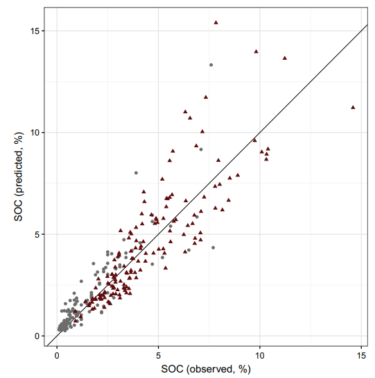
Note that in the previous equation, the fraction is the ratio of the residual sum of squares to the total data sum of squares. The residuals represent the difference between the prediction and reality. The closer R2 is to 1, the better the prediction. In a bivariate plot presenting the real values of the validation dataset on the abscissa axis and the predicted values of the validation dataset on the ordinate axis, one expects a linear regression to fit to most of the observations (Fig 1).

Figure 1. Goodness of fit (Predicted VS Real values). SOC is the Soil Organic Carbon content
However, it is necessary to be careful when calculating this determination coefficient because it may lead to erroneous conclusions. Indeed, some points of influence can particularly increase the value of the coefficient of determination, which can sometimes suggest that the predictions are quite accurate. Here, the model is relatively well fitted to the data. Grey dots close to the origin of the graph nevertheless help to increase the value of the determination coefficient.
The bias
The bias enables to evaluate whether predictions are accurate and also whether the model tends to over- or underestimate the values of the variable of interest. The computation is as follows :
Bias=\dfrac{\sum_{i=1}^{n}(\hat{y_i}-y_i)}{n}
Where y_i is the value of the ith observation in the validation dataset and \hat{y_i} is the predicted value for the ith observation.
The smaller the bias (closer to 0), the better the prediction. Be aware that this indicator does not account for the variability of the predictions. Indeed, if the predicted values are at the same time largely over and underestimated, the bias can still be relatively low.
To visually assess whether the predicted values are under or overestimated, one could plot the same bivariate plot as before and add the first bisector of the plot. In fact, if observations are located on this bisector, it means that the predicted values are equal to the real values. If they are below the line, predictions are always lower than the real values (predicted values are underestimates). The contrary applies when observations are located above the line.
The mean absolute error : MAE
MAE=\dfrac{\sum_{i=1}^{n}\mid\hat{y_i}-y_i\mid}{n}
Where y_iis the value of the ith observation in the validation dataset qnd \hat{y_i} is the predicted value for the ith observation.
The only difference between the MAE and the Bias is the absolute value of the differences between the real and the predicted values. One strong advantage of the MAE is that it gives a better idea of the prediction accuracy. However, it is not possible to know if the model tends to over or underestimate the predictions.
The root mean square error : RMSE
RMSE=\sqrt{\dfrac{\sum_{i=1}^{n}(\hat{y_i}-y_i)^2}{n}}
One last useful metric is the RMSE. It provides an indication regarding the dispersion or the variability of the prediction accuracy. It can be related to the variance of the model. Often, the RMSE value is difficult to interpret because one cannot tell whether a variance value is low or high. To overcome this issue, it is more interesting to normalize the RMSE so that this indicator can be expressed as a percentage of the mean of the observations. It can be used to make the RMSE more relative to what is being studied.
For instance, a RMSE of 10 is relatively low if the mean of the observations is 500. However, the model has a high variance if it generates a RMSE of 10 for an observations mean of 15. Indeed, in the first case, the variance of the model only reaches 5% of the mean while it reaches more than 65% of the mean in the second case.
None of these aforementioned indexes is definitely better than the others. On the contrary, all the metrics must be used in conjunction to provide a better understanding of the prediction accuracy.
Bias-variance trade-off

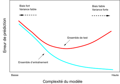
Figure 2. Bias and Variance Tradeoff. The training (“Ensemble d’entraintement”) and test (or validation) datasets are presented in the next section. [Complexité du modèle –> Model complexity; Erreur de prédiction –> Prediction error]
Figure 2 illustrates the tradeoff between the bias and variance of a model. In this figure, the bias is related to the accuracy of the model while the variance can be understood as the precision of the model. When creating a model, the objective is to have the lowest bias and variance possible to ensure the best possible estimations. However, it is relatively difficult to lower at the same time both parameters. Effectively, increasing the variance results in a decrease of the bias. On the other hand, increasing the bias leads to a decrease of the variance.
Bias and variance also have to do with the quality of fit of the model. It can be said that a model with a small variance and a high bias will tend to underfit the data. Indeed, it means that the predictions will not be very accurate but that multiple realizations of the model will lead to similar estimates. In other words, the model is not that specific to the data under study. On the contrary, a model with a large variance and a small bias overfits the data. In this case, the model is very specific to the data under study because it generates very accurate predictions for this particular dataset. However, when applying the model to another dataset (another application of the model), estimates will strongly differ from the real values because the model has not the ability to account for new observations. Overfitting is a common problem because models are generally created to fit relatively well to the samples available. When the model is confronted to another set of independent observations, it generates unreliable results. This is why it is fundamental to create a model with a training dataset and to validate it on a set of independent observations with regard to the training dataset. Models should be relatively flexible so that they are able to predict the value of an observation that is not too similar to the observations that were used to infer the model at first.
Cross-validation procedures
As previously stated, the validation of a predictive model requires to (i) divide a initial sample set into a training and validation datasets, (ii) infer a model with the training dataset, (iii) evaluate the quality of the model with the validation dataset by computing the aforementioned metrics. To ensure that the quality of the model is well estimated, these three steps must be repeated several times. Indeed, the initial dataset can be separated into lots of different training and validation datasets.
For instance, at the first iteration, the 70 % of observations that will be used in the training dataset will be different from the 70% of observations of the training dataset in the second iteration.
The validation metrics can be averaged over all the iterations to have a better characterization of the model. This concept is known as cross-validation because one checks whether the validation is similar among different training and validation datasets. At the beginning of the post, it was said that the training set generally involved between 60 and 80% of the initial dataset. If the validation dataset is set to contain 20% of the observations and multiple iterations are run, it is said that a 20-fold cross validation is being performed. If the validation dataset contains 5% of the observations, it is a 5-fold cross validation. Another commonly reported method is the leave one out cross validation. As the name suggests, the validation dataset is only made of one observation.
Validating a predictive model is necessary to ensure that a model is effectively able to predict accurately the values of a variable of interest. Once again, be aware that a model will be best evaluated with independent and relatively large training and validation datasets. It happens that some people use small and non independent dataset (some even validate their model with the observations that were used to create the model….) for the validation process in order to boost their validation metrics. It is recommended to run cross-validation procedures and to compute the mentioned validation metrics so that a predictive model is correctly evaluated.
Support Aspexit’s blog posts on TIPEEE
A small donation to continue to offer quality content and to always share and popularize knowledge =) ?

