Yield maps in Precision Agriculture

Table of contents

Share this article!

This post should have been published a long time ago, especially since it was the subject of my thesis. It’s now done…

First of all, one might ask why a thesis work was proposed on yield data when yield sensors have been around since the 1990s? First, it is clear that yield information is in itself of primary interest to producers. Yield does indeed quantify the level of production in a field and can be easily related to the gross margin of the farm (this will be the subject of a future post). Secondly, from a more general point of view, yield sensors have been available since the early 1990s, which means that historical yield mapping databases are likely to be available on many plots. It might therefore be interesting to return to this yield information with all the knowledge and feedback potentially available. We had imagined that rethinking the processing and analysis of this data by linking it to all the expert knowledge that has been gathered could help generate new information and perhaps raise new relevant questions and perspectives. It should also be noted that the yield map can be seen as a symbol of Precision Agriculture. Knowing that yield sensors were born over two decades ago but are still struggling to be used properly by field operators may also call into question the legitimacy of Precision Agriculture to meet the demands of professionals.

Yield monitors: one of the pioneer sources of PA

Yield monitors have been available since the early 1990’s. They have been key in the development of Precision Agriculture because they were one of the first means to define, quantify, and characterize the within-field variability in crop production

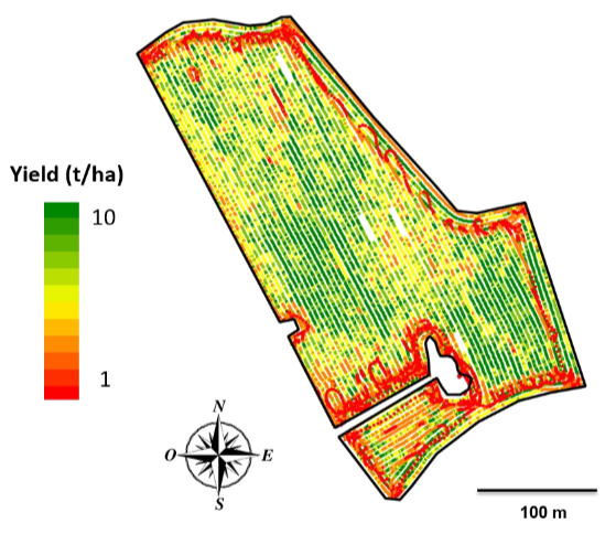
Figure 1. Yield map showing the within-field yield spatial variability

These monitors are mounted on combine harvesters and measure in real-time the amount of grain that passes through the combine when the crop is being harvested. Note that the type of yield measurement that is performed depends on the location of these sensors inside the machine. When the combine passes through the field, the crop (stems and grains) is cut at the header level and flows in the combine through the feed conveyer. The threshing systems then separate the grains from the stems. Grains are cleaned with the fan and sieve tables and work their way to the storage tank, the hoper, flowing through the grain auger trough and grain elevator. Stems are rejected from the combine.

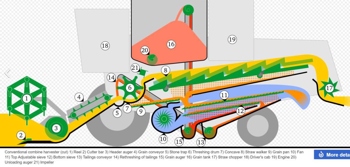
Figure 2. Diagram of a conventional combine harvester (Source : Wikipédia).

Acquisition of within-field yield data: combine harvesters and yield monitors

Yield monitors are usually installed near the grain elevator (Figure 3). Two main systems are usually reported: the volume-flow meters (Figure 3, a, b) and mass-flow meters (Figure 3, c, d,e,f) [Berducat, 2000; Chung et al., 2017].

Volume-flow sensors estimate the volume of grain either on a paddle wheel situated right after the grain elevator (Figure 3, a) or directly within the grain elevator using a one-way light barrier (Figure 3, b). In the first case, a level sensor measures the level of grain that is flowing through the wheel. In the second case, the volume of grain is estimated by the duration of light interruption as the grain flows through the grain elevator. Grain volumes are then converted into grain mass using the specific weight of the grain.

Mass-flow sensors rely either on the force measurement principle (Figure 3 , d,e,f) or on the absorption of gamma rays by mass (Figure 3, c) (Kormann et al., 1998 ). In the first case, the grain weight is estimated using a force transducer that measures the impact force of the grain at the end of the grain elevator. In the second case, a radiation detector measures the absorption of gamma rays (emitted by the radiat ion source) by the grain, which is then used to estimate the grain weight.

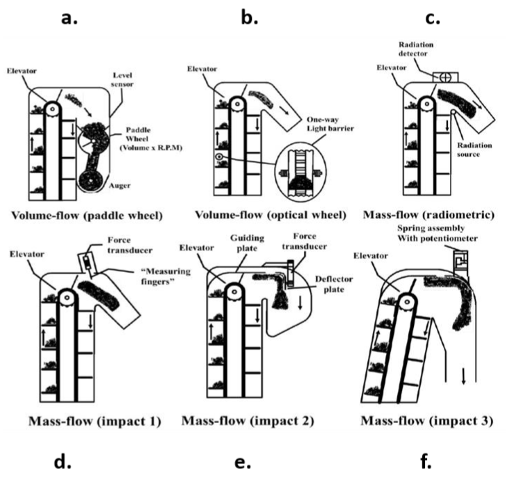
Figure 3. Yield monitors: mass and volume-flow sensors (source: Kormann et al., 1998)

All the combine harvester’s systems that come into play to calculate the crop yield are displayed in Figure 4. Moisture sensors are used to provide a yield record at a reference moisture level. These sensors are generally placed near the grain auger or grain elevator to estimate the grain moisture using the dielectric properties of the harvested grain. Note that the positioning systems enable to associate a location in space to yield records and consequently enable to generate yield maps.

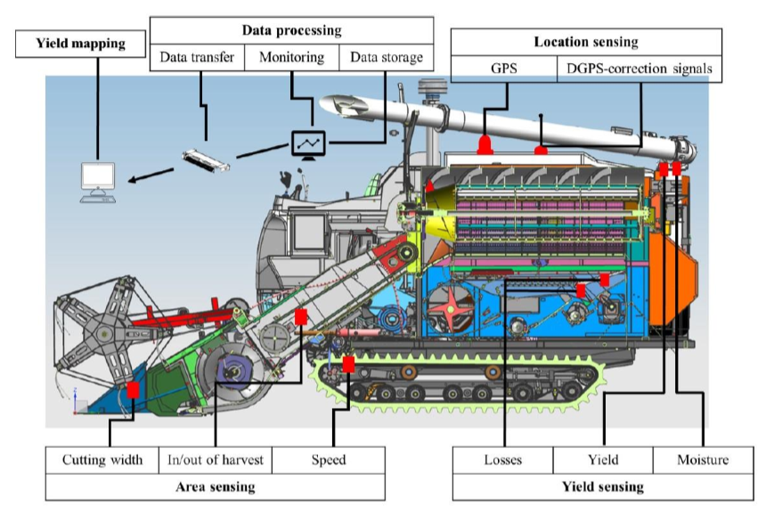
Figure 4. Yield mapping technologies within a combine harvester (source: Kormann et al., 1998; Chung et al., 2017)

Characteristics of within-field data

The acquisition of within-field yield data can be understood as a sequential procedure through time during which a combine acquires yield spatial information. T he data collection process follows a temporal dynamic, i.e., observations are recorded in a specific order one at a time as the machine passes through the field (Figure 5). The machine can simply be modelled by a structuring element that moves through the field, i.e., a rectangle whose dimensions are defined by the characteristics of the combine and the associated on-board sensors (yield monitor in this case). On-the-go yield measurements are punctual observations and each point synthesizes the yield response over the corresponding structuring element. The yield spatial resolution is controlled by the distance between consecutive records and determined by the distance between adjacent passes of the machine. The spatial distance between consecutive observations is related to the speed of the machine and the sampling frequency of the sensor . In a given field, this frequency of acquisition is generally stable, meaning that the distance between consecutive records only relies on the travel speed of the combine. On the other hand, when a combine harvester with an on-board grain yield monitor passes through a field, the distance between adjacent passes is related to the width of the cutting bar because the whole field has to be harvested.

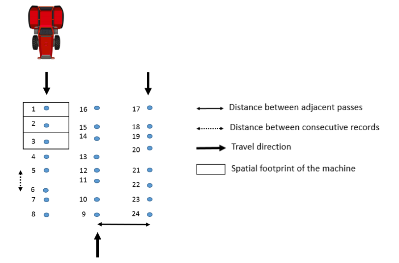
Figure 5. Acquiring within-field yield data (blue dots) with a combine harvester (source: Leroux et al., 2018a)

These observations are therefore irregularly-distributed in space because

the intra-row and inter-row distances are different and
(ii) the acquisition conditions, such as the GNSS accuracy or variable combine speed, can impact the spatial distribution of the observations, and
(iii) some observations can be missing (loss of positioning signal, full memory card).

The yield information is also very dense (thousands of points per hectare) and very noisy because of stochastic error in sensor operation, the intrinsic local variab ility in production and errors associated with the combine harvester passing through the field (Simbahan et al., 2004; Sudduth and Drummond, 2007). Nevertheless, within-field yield data usually exhibit quite a strong spatial structure, i.e., spatial observations are well-structured within the fields and yield spatial patterns are clearly visible (Pringle et al., 2003). As most arable crops need to be harvested each year, historical databases of yield mapping are likely to be available on many arable systems. However, it must be said that temporal within-field yield data might not be collocated in space (the yield monitor is not measuring the yield information at the exact same location each year)

Provision and usages

In the Precision Agriculture scientific community, yield data are generally used to (i) quantify and characterize within-field variability, (ii) correlate the yield with an auxiliary variable, and (iii) validate the suitability of a modulation application. And it should be said that it is not very complicated to find research that uses these within-field yield data at some point in time. Nevertheless, a recent scientific mapping study (a kind of mind-map) also showed that the interest of the precision farming scientific community in yield maps had decreased between the periods 2000-2009 and 2010-2016 (Pallottino et al., 2017).

When one is interested in the use of yield sensors in the field, it is another matter… There are already almost no statistics for France (this is why the French observatory of digital uses in France will soon release an infography on the subject). Nevertheless, more or less recent statistics for a number of countries – other than France – can be found in technical reports and scientific bibliography. I invite you to take these statistics with a little hindsight!

First of all, we must be clear on the fact that these trends in use vary greatly between countries (and sometimes even regions) and the cultures being monitored. American farmers may have been the first users to engage themselves in such yield mapping technologies (Griffin et al., 2004; Fountas et al. , 2005). These authors have reported that, by 2005, about 90% of yield monitors in the world were in the US. Griffin and Erickson (2009) have also provided some adoption rates from an Agricultural Resource Management Survey . According to the study and available data, 28% of U.S. corn planted acres (in 2005), 10% of winter wheat (in 2004), and 22% of soybeans (in 2002) were harvested with a combine equipped with a yield monitor. Norwood and Fulton (2009) have concluded in their study that 32% of US farmers w ere using yield monitoring systems. Figure 6 displays the results of another study investigating the adoption of yield mapping systems per crop in United States (Schimmelpfennig, 2016) . Even if the estimates are not exactly the same, trends can be considered similar. Regarding the investigated crops, it clea rly appears that the production of crops such as corn, soybean and wheat has been increasingly followed by farmers from the beginning of 2000’s through yield mapping technologies. Given the observed trends, the adoption in more recent campaigns (2017, 2018 ) should be expected to be again higher. A more recent study also stated the fact that rice farms in USA had been largely adopting yield monitoring technologies, by more than 60% (USDA, 2015).

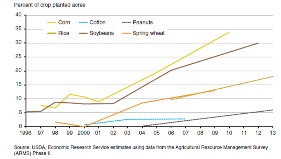
Figure 6. Adoption of yield mapping technologies per crop in United States

Adoption rates of yield mapping technologies are not as widely reported in other countries, but some national studies intended to provide some detailed numbers. According to the Department for Environment, Food & Rural Affairs, English farmers have experienced a small increase in yield mapping adoption from 7 to 11% between 2009 and 2012 (DEFRA, 2013). In Australia, McCallum and Sargent (2008) have reported a very low adoption rate of yield mapping tech nologies (less than 1%). Within the same country, it was estimated that about 800 yield monitors had been used in the 2000 harvest year (Mondal & Basu, 2009). Fountas et al. (2005) have evaluated that About 400 Danish, 400 British, 300 Swedish and 200 German farmers had adopted yield monitors by the year 2000. Yield mapping technologies have also been reported in developing countries (Say et al., 2017). In Argentina, Mondal and Basu (2009) have reported that about 4% of the grain and oil seed area had been harvested by combines with yield monitors in 2001 (560 yield monitors were in use). According to Keskin and Sekerli (2016), about 500 combine harvesters (3% countrywide) are equipped with yield monitoring systems in Turkey farms. Akdemir (2016) provided a lower adoption rate of yield mapping technologies (310 combines instead of 500) in the same country.

Advantages and limits of within-field yield data

While it is clear that the adoption of yield mapping technologies is increasing in both developed and developing countries, one may wonder which factors and aspects of within-field yield data may have contributed to such a slow adoption of yield mapping technologies. Yield monitors mounted on combine harvesters have been available since the early 1990’s. How ever, yield data still have difficulties in being a decisive component of the decision-making process in precision agriculture studies. In terms of the utility of yield data, multiple issues have been reported by the scientific community. First of all, it is clear that spatial yield patterns originate from an interaction between, management, climate and environmental (soil, landscape, pest attacks, etc) conditions within a cropping season, which means that it is not possible to derive variable-rate applicat ion maps directly for a year n by solely relying on yield data in year n-1. Secondly, it is acknowledged that in annual and perennial crops, the yield temporal variability is often stronger than the yield spatial variability, which can hinder analyses over short and long-time periods (Blackmore et al., 2003; Bramley and Hamilton, 2004; Eghball and Power, 1995; Lamb et al., 1997). This temporal variability is essentially due to non-stable factors, such as climate patterns or the type of crops being grown eac h year (Basso et al., 2012). Multiple authors have stated that the number of years of yield data available to conduct yield temporal analyses was critical (Bakhsh et al., 2000; Kitchen et al., 2005) and some have even tried to propose a minimum number of y ears necessary to obtain reliable results (Ping and Dobermann, 2005). On top of that, yield data often come with a large number of defective observations resulting from the pass of the combine harvester inside the fields, which do not correspond to the yield that should have been obtained under the growing conditions in the field (this will be discussed in the next post). Some of these erroneous observations are widely reported in the literature, e.g., flow delay, filling and emptying times, abrupt speed changes or partially-used cutting bar (Arslan and Colvin, 2002; Sudduth and Drummond, 2007). Some improvements have been proposed, e.g., sensors to measure in real-time the cutting width (Zhao et al., 2010), but most of the combines are not equipped with these new technologies. These errors, if not accounted for, can influence agronomical decisions over the fields (Griffin et al., 2008). From a more practical perspective, it can also be argued that end-users can solely get the yield information at the end of the growing season, which might constitute a limitation in terms of decision support tool.

However, from a precision agriculture standpoint, these high-resolution yield data are a very valuable source of information that would be aberrant not to consider (Florin et al., 2009). Yield spatial patterns are a valuable piece of information to better characterize the sources of spatial variability across the fields. Farmers are interested to know about the mean yield spatial and temporal patterns over their fields so they can make informed and reliable management decisions. It has been shown that, despite a strong temporal variability, it was often possible to detect consistent yield spatial patterns across years (Kitchen et al., 2005; Taylor et al., 2007). Some yield patterns were found consistent even under different crops and varying climate conditions. Furthermore, yield spatial patterns can deliver relevant information with respect to soil characteristics within the field or can help depict the influence of other external factors, such as managemen t practices and weather conditions (Diker et al., 2004). For instance, Taylor et al. (2007) showed that, in specific portions of their field study, crop rotation management in previous years originated variations in yield spatial patterns. Other authors have found that high-yielding areas in dry years could, at the same time, be low-yielding areas in wet years which could give critical information with respect to within-field soil characteristics (Colvin et al., 1997; Sudduth et al., 1997; Taylor et al., 20 07). Another strong advantage of these yield datasets is their accessibility. Something that was considered as a flaw in the previous paragraph can also be seen as a strong asset. Indeed, in most cases, harvest has to be made which means that these data can be collected yearly once farmers have invested in yield monitors , and consequently that large databases of yield mapping can be built. Finally, it should be argued that within-field yield data are directly related to the crop performance and so to the gross margin of the field . As such, these data bring a very comprehensible and practical information to farmers and advisors.

How to valorize yield maps?

Without going into the details of all the projects that could be carried out using yield maps, here is a small outline of what could be done. Some of these ideas have been addressed in the thesis manuscript that you will find on the website. Some of these ideas are quite operational, others are more exploratory. The list is obviously not exhaustive!

Spatialize agronomic models with high-resolution yield data. For example, work had been done on P/K fertilization plans to assess the extent to which within-field yield information could be used to refine fertilization plans, including refining within-field yield potentials and within-field P/K exports.
Spatialize performance/economic profitability maps on farms (this will be the subject of a forthcoming post)
Use yield time series to better understand yield potentials and within-field yield gaps. This work was addressed in the framework of the thesis
Evaluate the potential of modulation actions in a plot of land
Validate the relevance of field experiments
Improve knowledge of the yield at a given spatial scale (region, territory, etc.) for a cooperative or an elevator that would like to obtain supplies.
Use yield maps to guide field sampling campaigns
Use yield time series to improve understanding of yield limiting factors in the plots. Leads were evoked during the discussion of the thesis manuscript.
Use yield time series to assess the risk to a farmer of not changing his practices or not engaging in modulation or Precision Farming practices. Leads were evoked during the discussion of the thesis manuscript.

– ….

One last criticism for manufacturers.

We’ve just talked about accessibility of yield data; let’s talk about interoperability. If you start working with yield data, you’re going to realize very quickly that there are an impressive amount of data formats provided by manufacturers…. But these are mostly private formats ! If you don’t have the proprietary software that goes with it, good luck… You will then have to develop specific modules to be able to read them. Add to that the fact that each constructor measures the variables that interest him, and that the units of measurement are different and you will tear your hair out pretty quickly.

Manufacturers, if you read this post, make your data accessible in an open, free or at least standardized format!

You’ll excuse me for the bibliographical references that I didn’t reclassify specifically for this post… but you should be able to find them without any problem =)

Acevedo-Opazo, C., Tisseyre, B., Guillaume, S., & Ojeda, H. (2008). The potential of high spatial resolution information to define within-vineyard zones related to vine water status. Precision Agriculture, 9, 285-302.
Adams, R., & Bischof, L. (1994). Seeded Region Growing. IEEE Transactions on Pattern Analysis and Machine Intelligence, 16, 641-647
Akdemir, B. (2016). Evalution of precision farming research and applications in Turkey. VII International Scientific Agriculture Symposium “Agrosym 2016”. 6-9 October 2016, Jahorina, Bosnia and Herzegovina. Proceedings Book. pp.1498-1504.
Angiulli, F., Fassetti, F., & Palopoli, L. (2009). Detecting outlying properties of exceptional objects. ACM Transactions on Database Systems, 34, 1, 1-7.
Angiulli, F., Fassetti, F., & Palopoli, L. (2012). Discoverying characterizations of the behavior of outlier sub -populations. IEEE Transactions on Knowledge and Data Engineering, 25, 1280-1292
Arslan, S., & Colvin, T. (2002 ). Grain yield mapping : yield sensing, yield reconstruction, and errors. Precision Agriculture, 3, 135-154
Arslan, S. (2008). A Grain Flow Model to Simulate Grain Yield Sensor Response. Sensors, 8, 952–962.
Arun, P.V. (2013). A comparative analysis of different DEM interpolation methods. The Egyptian Journal of Remote Sensing and Space Science, 16, 2, 133-139.
Baluja, J., Diago, M., Goovaerts, P., & Tardaguila, J. (2012 ). Assessment of the spatial variability of anthocyanins in grapes using a fluorescence sensor: relationships with vine vigour and yield. Precision Agriculture, 13, 457–472.
Bakhsh, A., Jaynes, D.B., Colvin, T.S., & Kanxar, R.S. (2000). Spatio-temporal analysis of yield variability for a corn-soybean field in Iowa. Agricultural and Biosystems Engineering, 43, 31-38.
Barnaghi, P., Sheth, A., & Henson C. (2013 ) “From data to actionable knowledge: Big data challenges in the web of things,” Intelligent Systems, IEEE, 28, 6–11, 2013.
Basso, B., Bertocco, M., Sartori, L., & Martin, E.C. (2007 ). Analyzing the effects of climate variability on spatial pattern of yield in a maize–wheat–soybean rotation. European Journal of Agronomy, 26, 82–91.
Basso, B., Fiorentino, C., Cammarano, D., Cafiero, G., & Dardanelli, J. (2012 ). Analysis of rainfall distribution on spatial and temporal patterns of wheat yield in Mediterranean environment. European Journal of Agronomy, 41, 52-65.
Basso, B., B. Dumont, D. Cammarano, A. Pezzuolo, F. Marinello, & L. Sartori. (2016 ). Environmental and economic benefits of variable rate nitrogen fertilization in a nitrate vulnerable zone . Science of the Total Environment. 545–546, 227–235
Bellehumeur, C., Legendre, P., & Marcotte, D. (1997). Variance and spatial scales in a tropical rain forest: changing the size of sampling units. Plant Ecology, 130, 89-98.
Ben-Gal, I. (2005 ). Outlier Detection. The Data Mining and Knowledge Discovery Handbook: A Complete Guide for Practitioners and Researchers. Boston: Kluwer Academic Publishers.
Berducat, M., Boffety, D. (2000). Gestion de l’information parcellaire – cartographie du rendement à la récolte. Ingénieries – E A T, IRSTEA édition 2000, p. 53 – p. 62
Beyer, K., Goldstein, J., Ramakrishnan, R., & Shaft, U. (1999). When is nearest neighbor meaningful ? In Proceedings of the 7 th ICDT, Jerusalem, Israel.
Bivand R.S., Pebesma, E.J., & Gomez-Rubio, V. (2008). Applied Spatial Data Analysis with R. New York, NY: Springer
Blackmore, B. S., & Moore, M. (1999). Remedial correction of yield map data. Precision Agriculture, 1, 53 – 66.
Blackmore, S., Godwin, R.J., & Fountas, S. (2003 ). The analysis of spatial and temporal trends in yield map data over six years. Biosystems Engineering. 84, 455-466.
Bongiovanni, B. and Lowenberg-Deboer, J. (2004). Precision agriculture and sustainability. Precision Agriculture, 5, 359_387.
Bongiovanni, R.G., Robledo, C.W., & Lambert, D.M. (2007). Economics of site-specific nitrogen management for protein content in wheat. Computers and Electronics in Agriculture, 58, 13–24.
Bramley, R.G.V., & Hamilton, R.P. (2004). Understanding variability in winegrape production systems. Australian Journal of Grape and Wine Research, 10, 32–45
Bramley, R.G., Hill, P.A., Thorburn, P.J., Kroon, F.J., & Panten, K (2008 ). Precision agriculture for improved environmental outcomes: some Australian perspectives. Agriculture Forest Research, 3, 161–178.
Breunig, M.M., Kriegel, H.P., Ng, R.T., & Sander, J. (2000). Lof: identifying density-based local outliers. In Proceedings of 2000 ACM SIGMOD International Conference on Management of Data. ACM Press, pp. 93 – 104
Cambardella, C.A., Moorman, T.B., Novak, J.M., Parkin, T.B., Karlen, D.L., Turco, R.F. et al. (1994). Field -scale variability of soil properties in central Iowa soils. Soil Science Society of America Journal, 58, 1501 – 1511.
Cambardella, C. A., & Karlen, D. L. (1999). Spatial analysis of soil fertility parameters. Precision Agriculture, 1, 5-14.
Cao, Q., Cui, Z., Chen, X., Khosla, R., Dao, T.H., & Miao, Y. (2012 ). Quantifying spatial variability of indigenous nitrogen management in small scale farming. Precision Agriculture, 13, 45–61.
Cassman, K. G. (1999 ). Ecological intensification of cereal production systems: yield potential, soil quality, and precision agriculture. Proceedings of the National Academy of Sciences of the United States of America , 96, 5952–5959
Cerovic, Z.G., Goutouly, J.P., Hilbert, G., Destrac-Irvine, A., Martinon, V., & Moise, N. (2009 ) Mapping winegrape quality attributes using portable fluorescence-based sensors. In: Best S (ed) Progap INIA, FRUTIC 09, Conception, Chile, pp 301–310
Chen, D., Lu, C-T., Kou, Y. & Chen, F. (2008). On Detecting Spatial Outliers. Geoinformatica, 12, 455-475
Chung, S. O., Sudduth, K. A., & Drummond, S. T. (2002 ). Determining Yield Monitoring System Delay Time With Geostatistical and Data Segmentation Approaches. Transactions of the ASAE, 45, 915-926.
Chung, S.O., Choi, M.C., Lee, K.H, Kim, Y.J, Hong, S.J., Li, M. (2016 ). Sensing Technologies for Grain Crop Yield Monitoring Systems: A Review. Journal of Biosystems Engineering, 41, 408-417.
Cid-Garcia, N.M., Albornoz, V., Rios-Solis, Y.A., & Ortega, R. (2013 ). Rectangular shape management zone delineation using integer linear programming. Computer and Electronics in Agriculture, 93, 1–9.
Clifford, P., Richardson, S., & Hemon, D. (1989 ). Testing the association between two spatial processes. Biometrics, 45, 123–134.
Collins, E.D., & Chandrasekaran, K. (2012 ). A Wolf in Sheep’s Clothing? An Analysis of the ‘Sustainable Intensification’ of Agriculture (Friends of the Earth International, Amsterdam, 2012)
Colvin, T.S., Jaynes, D.B., Karlen, D.L., Laird, D.A., & Ambuel, J.R. (1997 ). Yield variability within a central Iowa field. Transactions of the ASAE, 40, 883–889.
Comifer (2007 ). Teneur en P, K et Mg des organes végétaux récoltés pour les cultures de plein champ et les principaux fourrages, Comifer, Paris, 6 pages.
Cox, S. (2002). Information technology : the global key to precision agriculture and sustainability. Computers and Electronics in Agriculture, 36, 93-111.
Cressie, N. A., (1991). Statistics for Spatial Data. John Wiley & Sons, New York.
Cressie, N. (1996). Change of support and the modifiable areal unit proble. Geographical Systems, 3, 159 – 180
Dale, M.R.T, & Fortin, M.J. (2002). Spatial autocorrelation and statistical tests in ecology. Eco Science , 9, 162-167
Davatgar, N., Neishabouri, M.R., & Sepaskhah, A.R. (2012 ). Delineation of site specific nutrient management zones for a paddy cultivated area based on soil fertility using fuzzy clustering. Geoderma, 173–174, 111–118.
Debuisson, S., Germain, C., Garcia, O., Panigai, L., Moncomble, D., Le Moigne, et al. (2010 ). Using Multiplex® and Greenseeker™ to manage spatial variation of vine vigor in Champagne. 10th International Conference on Precision Agriculture.
de Oliveira, R. P., Whelan, B. M., McBratney, A. B., & Taylor, J. A. (2007 ). Yield variability as an index supporting management decisions: YIELDex. Proceedings of the 6th European Conference on Precision Agriculture, 281–288.
DEFRA (2013). Farm Practices Survey Autumn 2012 – England. Department for Environment, Food and Rural Affairs (DEFRA). 41pp.
Di Virgilio, N., Monti, A., & Venturi, G. (2007). Spatial variability of switchgrass (Panicum virgatum L.) yield as related to soil parameters in a small field. Field Crops Research, 101, 232-239.
Diker, K., D.F. Heerman, & M.K. Brodahl. (2004 ). Frequency analysis of yield for delineating yield response zones. Precision Agriculture, 5, 435–444.
Drummond, S. T., Fraisse, C. W., & Sudduth, K. A. (1999 ). Combine Harvest Area Determination by Vector Processing of GPS Position Data. Transactions of the ASAE, 42, 1221–1227.
Duan, L., Xu, L., Guo, F., Lee, J., & Yan, B. (2007). A local-density based spatial clustering algorithm with noise. Information Systems, 32, 978–986
Duan L., Tang, G., Pei, J., Bailey, J., Campbell, A., & Tang, C. (2015 ). Mining outlying aspects on numeric data. Data Mining Knowledge Discovery, 29, 1116–1151
Dutilleul, P. (1993). Modifying the t-test for assessing the correlation between two spatial processes. Biometrics, 49, 305–314.
Eghball, B., Power, J.F. (1995). Fractal description of temporal yield variability of 10 crops in the United States. Agronomy Journal, 87, 152-156.
Ertoz, L., Eilertson, E., Lazarevic, A., Tan, P., Srivastava, J., Kumar, V., & Dokas, P. (2004). The MINDS – Minnesota Intrusion Detection System, in Data Mining, A. Joshi H. Kargupta, K. Sivakumar, and Y. Yesha (Eds.) Next Generation Challenges and Future Directions.
Ester, M., Kriegel, H.-P., Sander, J., & Xu, X. (1996). A density-based algorithm for discovering clusters in large spatial databases with noise. In E. Simoudis, J. Han, and U. Fayyad (Eds.), Proceedings of Second International Conference on Knowledge Discovery and Data Mining , Palo Alto, CA, USA: AAAI Press, pp 226–231.
European Parliamentary Research Service (2016 ). Precision Agriculture and the Future of Farming in Europe, STOA, Brussels, European Union.
EU SCAR. (2012). Agricultural knowledge and innovation systems in transition. Brussels: EU.
Fairfield Smith, H. (1938). An empirical law describing heterogeneity in the yield of agricultural crops. The Journal of Agricultural Science, 28, 1–23.
FAO (2017). The future of food and agriculture. http://www.fao.org/3/a-i6644e.pdf (accessed 05/06/2018)
Fauvel, M., Chanussot, J., & Benediktsson, J.A. (2011). A spatial–spectral kernel-based approach for the classification of remote-sensing images. Pattern Recognition, 45, 381-392.
Fauvel, M., Tarabalka, Y., Benediktsson, J.A., Chanussot, J., & Tilton, J. (2012). Advances in Spectral-Spatial Classication of Hyperspectral Images. Proceedings of the IEEE, Institute of Electrical and Electronics Engineers, 101, 652-675.
Filzmoser, P., Ruiz-Gazen, A., & Thomas-Agnan, C. (2014). Identification of local multivariate outliers. Statistical Papers, 55, 29-47.
Florin, M.J., McBratney, A.B., & Whelan, B.M. (2009 ). Quantification and comparison of wheat yield variation across space and time. European Journal of Agronomy, 30, 212-219.
Fountas, S., Pedersen, S.M., & Blackmore, S. (2005). ICT in Precision Agriculture – diffusion of technology. In “ICT in Agriculture: Perspectives of Technological Innovation” edited by E. Gelb, A. Offer. 15pp.
Fraisse, C.W., Sudduth, K.A., Kitchen, N.R. (2001). Delineation of site-specific management zones by unsupervised classification of topographic attributes and soil electrical conductivity. Transactions of the ASAE, 44, 155-166.
Fulton, J.P., Shearer, S.A., Chabra, G., & Higgins, S.F. (2001 ). Performance assessment and model development of a variable-rate, spinner-disc fertilizer applicator. Transactions of the ASAE, 44, 1071-1081.
Fulton, J. P., Shearer, S.A., Higgins, S.F., Darr, M.J., & Stombaugh, T.S. (2005 ). Rate response assessment from various granular VRT applicators. Transactions of the ASAE, 48, 2095‐2103.
Garnett, T., Appleby, M. C., Balmford, A., Bateman, I. J., Benton, T. G., Bloomer, P., et al. (2013 ). Sustainable intensification in agriculture: Premises and policies. Science, 341, 33–34.
Gogoi, P, Bhattacharyya D, Borah B, & Kalita JK (2011 ). A survey of outlier detection methods in network anomaly identification. Computer Journal, 54, 570–88.
Goldman Sachs (2016). Precision Farming. Cheating Malthus with Digital Agriculture. Profiles in Innovation.
Goovaerts P. (1997). Geostatistics for Natural Ressources Evaluation, Applied Geostatistics Series, Oxford University Press, New York.
Grassini, P., van Bussel, L.G.J., van Wart, J., Wolf, J., Claessens, L., Yang, H. et al. (2015 ). How good is good enough? Data requirements for reliable crop yield simulations and yield-gap analysis. Field Crops Research, 177, 49-63.
Griepentrog, H.W., Thiessen, E., Kristensen, H. & Knudsen, L. (2007). A patch-size index to assess machinery to match soil and crop spatial variability. In Proceedings: 6th European Conference on Precision Agriculture.
Griffin, T.W., Lowenberg-Deboer, J., Lambert, D.M., Peone, J., Payne, T., & Daberkow, S.G. (2004 ). Adoption, profitability, and making better use of precision farming data. Staff Paper #04-06. Department of Agricultural Economics, Purdue University.
Griffin, T., Dobbins, C., Vyn, T., Florax, R., & Lowenberg-DeBoer, J. (2008 ). Spatial analysis of yield monitor data: case studies of on-farm trials and farm management decision making. Precision Agriculture , 9, 269–283
Griffin, T. & Erickson, B. (2009 ). Adoption and Use of Yield Monitor Technology for U.S. Crop Production. Site Specific Management Center Newsletter, Purdue University, 9pp.
Grisso, R., Alley, M. & Groover, G. (2009). Precision Farming Tools: GPS Navigation. Virginia Cooperative Extension. Publication No 442-501. 7pp.
Han, S., J.W. Hummel, C.E. Goering, & M.D. Cahn. (1994). Cell size selection for site-specific crop management. American Society of Agricultural and Biological Engineers, 37, 19–26.
Haralick, R.M., Shanmugam, K., & Dinstein, I. (1973). Texture features for image classification, IEEE Transactions on Systems, Man and Cybernetics, 3, 610-621.
Harris, P., Brunsdon, C., Charlton, M., Juggins, S., & Clarke, A. (2014 ). Multivariate Spatial Outlier Detection Using Robust Geographically Weighted Methods. Math Geosciences, 1–31.
Hawkins, D. (1980). Identification of Outliers, London, UK: Chapman & Hall
Hu, J., Gong C., & Zhang Z. (2012) Dynamic Compensation for Impact-Based Grain Flow Sensor. In: Li D., Chen Y. (eds) Computer and Computing Technologies in Agriculture V. CCTA 2011. IFIP Advances in Information and Communication Technology, vol 370, 210-216, Berlin, Heidelberg, Germany: Springer
Hubert, M., & Van der Veeken, S. (2008). Outlier detection for skewed data. Journal of Chemometrics , 22, 235–246
Iqbal, J., Thomasson, J.A., Jenkins, J.N., Owens, P.R & Whisler, F.D. (2005 ). Spatial Variability Analysis of Soil Physical Properties of Alluvial Soils. Soil Science Society of America, 69, 1-14.
Jingtao, Q., & Shuhui, Z. (2010). Experiment research of impact-based sensor to monitor corn ear yield. International Conference on Computer Application and System Modeling, IEEE, 101, 187–192.
Jones, H., Guillaume, S., Loisel, P., Charnomordic, B., & Tisseyre, B. (2016). Generation of Plateau -Approximated Fuzzy Zones. In Proceedings of the Conference on Spatial Accuracy, Montpellier, France.
Journel, A. G., & Huijbregts, C. J. (1978). Mining geostatistics. Academic Press, London, England.
Junior, V.V., Carvalh, M.P., Dafonte, J., Freddi, O.S., Vidal Vazquez, E., & Ingaramo, O.E. (2006 ). Spatial variability of soil water content and mechanical resistance of Brazilian ferralsol. Soil and Tillage Research , 85, 166–177.
Keskin, M., & Sekerli, Y.E. (2016 ). Awareness and adoption of precision agriculture in the Cukurova region of Turkey. Agronomy Research, 14, 1307–1320.
Kitchen, N.R., Sudduth, K.A., Myers, D.B., Drummond, S.T., & Hong, S.Y. (2005). Delineating productivity zones on claypan soil fields using apparent soil electrical conductivity. Computers and Electronics in Agriculture, 46, 285-308
Knorr E. M., & Ng R. T. (1999). Finding Intensional Knowledge of Distance-based Outliers. In Proceeding s of the 25th International Conference on Very Large Data Bases, Edinburgh, Scotland, pp. 211-222
Koch, B., Khosla, R., Frasier, W.M., Westfall, D.G., & Inman, D. (2004). Economic feasibility of variable -rate nitrogen application utilizing site-specific management zones. Agronomy Journal, 96, 1572–1580
Kormann, G., Demmel, M., & Auernhammer, H. (1998). Testing stand for yield measurement systems in combine harvesters. ASAE;St. Joseph, MI: 1998. ASAE Paper No. 983102.
Kravchenko, A.N., Robertson, G.P., Thelen, K.D., & Harwood, R.R. (2005). Management, topographical, and weather eff ects on spatial variability of crop grain yields. Agronomy Journal, 97, 514–523.
Lachia, N. (2017 ). Usages de la télédétection en agriculture. Observatoire des usages de l’agriculture numérique. http://agrotic.org/observatoire/
Lamb, J.A., Dowdy, R.H., Anderson, J.L., & Rehm, G.W. (1997). Spatial and temporal stability of corn grain yields. Journal of Production Agriculture, 10, 410-414.
Larson, J.A., M.M. Velandia, M.J. Buschermohle, & S.M. Westland (2016 ). Effect of field geometry on profitability of automatic section control for chemical application equipment. Precision Agriculture, 17, 18 – 35.
Lauzon, J.D., Fallow, D.J., O’Halloran, I.P., Gregory, S.D.L., & von Bertoldi, A.P. (2005 ). Assessing the temporal stability of spatial patterns in crop yields using combine yield monitor data. Canadian Journal of Soil Science, 439-451.
Lee, D. H., Sudduth, K. A., Drummond, S. T., Chung, S. O., & Myers, D. B. (2012 ). Automated yield map delay identification using phase correlation methodology. Transactions of the ASABE, 55, 743–752.
Legendre, P. & L. Legendre (1998). Numerical Ecology, 2nd English edition. Elsevier, Amsterdam.
Leroux, C., Jones, H., Clenet, A., & Tisseyre, B. (2017a). A new approach for zoning irregularly-spaced, within-field data. Computers and Electronics in Agriculture, 141, 196-206.
Leroux, C., Jones, H., Clenet, A., Dreux, B., Becu, M., & Tisseyre, B. (2017b). Simulating yield datasets: an opportunity to improve da ta filtering algorithms. In J A Taylor, D Cammarano, A Preashar, A Hamilton (Eds.), Proceedings of the 11th European Conference on Precision Agriculture, Precision Agriculture ’17 (Advances in Animal Biosciences, 8, 600-605.
Leroux, C., Jones, H., Clenet, A., &Tisseyre, B. (2018a). A general method to filter out defective spatial observations from yield mapping datasets. Precision Agriculture. https://doi.org/10.1007/s11119-017-9555-0
Leroux, C., Jones, H., Taylor, J, Clenet, A., & Tisseyre, B. (2018b). A zone-based approach for processing and interpreting variability in multitemporal yield data sets. Computers and Electronics in Agriculture, 148, 299-308. https://doi.org/10.1016/j.compag.2018.03.029
Li, Y., Shi, Z., Li, F., & Li, H.Y. (2007). Delineation of site-specific management zones using fuzzy clustering analysis in a coastal saline land. Computer and Electronics in Agriculture, 56, 174–186
Lindblom, J., Lundström, C., Ljung, M., & Jonsson, A. (2016 ). Promoting sustainable intensifcation in precision agriculture: Review of decision support systems development and strategies. Precision Agriculture , 18, 309–331.
Loisel, P., Jones, H., Charnomordic, B., & Tisseyre, B. (2018). An optimisation-based approach to generate intepretable within-field zones. Precision Agriculture, https://doi.org/10.1007/s11119-018-9584-3
López-Granados, F., Jurado-Expósito, M., Atenciano, S., García-Ferrer, A., Sánchez de la Orden, M., & García-Torres, L. (2002). Spatial variability of agricultural soil parameters in southern Spain. Plant and Soil, 246, 97-105.
López-Granados, F., Jurado-Expósito, M., Alamo, S., & Garcıa-Torres, L. (2004). Leaf nutrient spatial variability and site-specific fertilization maps within olive (Olea europaea L.) orchards. European Journal of Agronomy, 21, 209-222.
Lu, C.-T., Chen, D., & Kou, Y. (2003). Algorithms for spatial outlier detection . In X.Wu, A. Tuzhilin, and J. Shavlik (Eds.) Proceedings of the Third IEEE International Conference on Data Mining , Los Alamitos, CA, USA: IEEE Press, pp 597-600.
Lyle, G., Bryan, B., & Ostendorf, B. (2013). Post-processing methods to eliminate erroneous grain yield measurements: review and directions for future development. Precision Agriculture, 15, 377-402.
Maine, N., Nell, W.T., Lowenberg-DeBoer, J., & Alemu, Z.G. (2010) Economic Analysis of Phosphorus Applications under Variable and Single-Rate Applications in the Bothaville District, Agrekon, 46, 532-547
Maini, R., & Aggarwal, H. (2009 ). Study and Comparison of Various Image Edge Detection Techniques. International Journal of Image Processing, 3, 1-11.
Marques, H.O., Campello, R.J., Zimek, A., Sander, J. (2015 ). On the internal evaluation of unsupervised outlier detection. In Proceedings of the 27th International Conference on Scientific and Statistical Database Management (SSDBM ’15), Amarnath Gupta and Susan Rathbun (Eds.), ACM, New York, NY, USA, 12 pp
Marques da Silva, J.R. (2006). Analysis of the Spatial and Temporal Variability of Irrigated Maize Yield. Biosystems Engineering, 94, 337–349
Massey, R.E., Myers, D.B., Kitchen, N.R., & Sudduth, K.A. (2008). Profitability maps as an input for site -specific management decision making. Agronomy Journal, 100, 52-59.
Matheron, G. (1963). Principles of geostatistics. Economic Geology, 58, 1246–1266
McCallum, M., & Sargent, M. (2008). The Economics of adopting PA technologies on Australian farms. 12th Annual Symposium on Precision Agriculture Research & Application in Australasia. The Australian Technology Park, Eveleigh, Sydney. 19 September 2008. p.44-47.
McBratney, A. & Taylor, J. (2000 ). PV or not PV? In Proceedings of the 5th International Symposium on Cool Climate Viticulture and Oenology, Melbourne, Australia.
McBratney, A., Whelan, B., Ancev, T., & Bouma, J. (2005). Future directions of precisi on agriculture. Precision Agriculture, 6, 7-23.
Mehnert, A., & Jackway, V. (1997). Improved seeded region growing algorithm. Pattern Recognition , Letters 18, 1065–1071.
Mercer, W. B., & Hall, A. D. (1911). The experimental error of field trials. Journal of Agricultural Science, 4, 107–132.
Molin, J.P. (2002 ). Methodology for identification, characterization and removal of errors on yield maps. ASAE Annual International Meeting, Chicago, Proceedings, Illinois.
Molin, J.P., & Faulin, G.D.C. (2002). Spatial an d temporal variability of soil electrical conductivity related to soil moisture. Scientia Agricola, 70, 1-5.
Molin, J. P., Menegatti, L.A.A, Pereira, L.L., Cremonini, L.C., & Evangelista, M. (2002 ). Testing a fertilizer spreader with VRT. In Proceedings of the World Congress of Computers in Agriculture and Natural Resources, 232-237
Mondal, P., & Basu, M. (2009 ). Adoption of precision agriculture technologies in India and in some developing countries: Scope, present status and strategies. Progress in Natural Science, 19, 659–666
Monsó, A., Arnó, J., & Martínez-Casasnovas, J.A. (2013). A simplified index to assess the opportunity for selective wine grape harvesting from vigour maps. Proceedings of the 9th European Conference on Precision Agriculture, 625-32
Moral F.J., Terron J.M., Marques da Silva, J.R. (2010). Delineation of management zones using mobile measurements of soil electrical conductivity and multivariate geostatistical techniques. Soil & Tillage Research, 106, 335–343
Norwood, S. & Fulton, J. (2009). GPS/GIS Applications for Farming Systems. Alabama Farmers Federation Commodity Organizational Meeting, USA.
Noyel, G., Angulo, J., Jeulin, D. (2007). Morphological segmentation of hyperspectral images. Image Analysis and Stereology, 26, 101-109.
Oliver, M.A., Webster, M. (1989 ). A geostatistical basis for spatial weighing in multivariate classification, Mathematical Geology, 21, 15-35.
Oliver, M. A. (2010). Geostatistical Applications for Precision Agriculture, Springer, London, UK, 295 pp.
Oliver, Y.M., & Robertson, M.J. (2013 ). Quantifying the spatial pattern of the yield gap within a farm in a low rainfall Mediterranean climate. Field Crops Research, 150, 29-41.
Özgöz, E., Günay, H., Önen, H., Bayram, M., & Acir, N. (2012 ). Effect of management on spatial and temporal distribution of soil physical properties. Journal of Agricultural Sciences, 18, 77–91.
Pal, N.R., & Pal, S.K. (1993). A review on image segmentation techniques. Pattern Recognition, 26, 1277 – 1294.
Pallottino, F., Biocca, M., Nardi, P., Figorilli, S., Menesatti, P., & Costa, C. (2017). Science mapping approach to analyze the research evolution on precision agriculture: world, EU and Italian situation. Precision Agriculture, https://doi.org/10.1007/s11119-018-9569-2
Paoli J. N., Tisseyre B., Strauss O., & McBratney A.B. (2010 ). A technical opportunity index based on a fuzzy footprint of the machine for site-specific management: application to viticulture. Precision Agriculture, 11(4) , 379-396.
Pedroso, M., Taylor, J., Tisseyre, B., Charnomordic, B., & Guillaume, S. (2010 ), A segmentation algorithm for the delineation of management zones, Computer and Electronics in Agriculture, 70, 199–208.
Peralta, N.R., Costa, J.L., Balzarini, M., Franco, M.C., Córdoba, M., & Bullock, D. (2015 ). Delineation of management zones to improve nitrogen management of wheat, Computer and Electronics in Agriculture . 110, 103–113.
Pham, D.L., Xu, C.Y., & Prince, J.L. (2000 ) A survey of current methods in medical image segmentation. Annual review of biomedical engineering, 315–337.
Ping, J.L., & Dobermann, A. (2003). Creating spatially contiguous yield classes for site-specific management. Agronomy Journal, 95, 1121–1131
Ping, J.L, & Dobermann, A. (2005). Processign of yield map data. Precision Agriculture, 6, 193-212.
Pringle, M. J., McBratney, A. B., Whelan, B. M., & Taylor, J. A. (2003 ). A preliminary approach to assessing the opportunity for site-specific crop management in a field, using a yield monitor. Agricultural Systems, 76, 273–292.
R Core Team (2013) R: A language and environment for statistical computing. R Foundation for Statistical Computing, Vienna, Austria.
Rab, M.A., Fisher, P.D., Armstrong, R.D., Abuzar, M., Robinson, N.J., & Chandra, S. (2009 ). Advances in precision agriculture in south-eastern Australia. IV. Spatial variability in plant-available water capacity of soil and its relationship with yield in site-specific management zones. Crop and Pasture Science, 60, 885-900
Reinke, R., Dankowicz, H., Phelan, J., & Kang, W. (2011 ). A dynamic grain flow model for a mass flow yield sensor on a combine. Precision Agriculture, 12, 732–749
Reitz, P., & H. D. Kutzbach (1996 ). Investigations on a particular yield mapping system for combine harvesters. Computers and Electronics in Agriculture, 14, 137–150.
Reza, S.K., Sarkar, D., Baruah, U., & Das, T.H. (2010 ) Evaluation and comparison of ordinary kriging and inverse distance weighting methods for prediction of spatial variability of some chemical parameters of Dhalai district, Tripura. Agropedology, 2, 38–48
Robert, P. C. (1993 ). Characterisation of soil conditions at the field level for soil specific management. Geoderma 60, 57–72.
Robert, P. C. (1999). Precision agriculture: research needs and status in the USA. In: Precision Agriculture, 99 Proceedings of the 2nd European Conference on Precision Agriculture, edited by J. V. Stafford (Sheffield Academic Press, Sheffield, UK), Part 1, p. 19–33.
Robertson, G.P., Klingensmith, K.M., Klug, M.J., Paul, E.A., Crum, J.R., & Ellis B.G. (1997 ). Soil resources, microbial activity, and primary production across an agricultural ecosystem. Ecological Applications, 7, 158 – 70
Robertson, M., Lyle, G., & Bowden, J. W. (2008). Within-field variability of wheat yield and economic implications for spatially variable nutrient management. Field Crops Research, 105, 211-220.
Robinson, T. P., & Metternicht, G. (2005). Comparing the performance of techniques to improve the quality of yield maps. Agricultural Systems, 85, 19–41
Rodeghiero, M., & Cescatti, A. (2008 ). Spatial variability and optimal sampling strategy of soil respiration. Forest Ecology and Management, 255, 106-112
Roland Berger Strategy Consultants (2016 ). Business opportunities in Precision Agriculture: Will Big Data feed the world in the future ? https://www.rolandberger.com/de/Publications/pub_precision_farming.html (accessed on 05/06/2018)
Roudier, P., Tisseyre, B., Poilvé, H., & Roger, J. (2008). Management zone delineation using a modified watershed algorithm. Precision Agriculture, 9, 233–250.
Roudier, P., Tisseyre, B., Poilvé, H., & Roger, J. (2011). A technical opportunity index adapted to zone specific management. Precision Agriculture, 12, 130–145.
Röver, M., & Kaiser, E. A. (1999). Spatial heterogeneity within the plough layer: low and mod erate variability of soil properties. Soil Biology and Biochemistry, 31, 175-187.
Sadras, V. & Bongiovanni, R. (2004 ). Use of Lorenz curves and Gini coefficients to assess yield inequality within paddocks. Field Crops Research, 90, 303–310
Santesteban, L. G., Guillaume, S., Royo, J. B., & Tisseyre, B. (2013 ) Are precision agriculture tools and methods relevant at the wholevineyard scale? Precision Agriculture, 14, 2–17.
Sawant, K. (2014). Adaptive methods for determining DBSCAN parameters. International Jou rnal of Innovative Science, Engineering & Technology, 1, 330-334
Say, M., Keskin, M., Sehri, M., & Sekerli, Y.E. (2017 ). Adoption of precision agriculture technologies in developed and developing countries. International Science and Technology Conference, July 17-19, Berlin
Schimmelpfennig, David (2016). Farm Profits and Adoption of Precision Agriculture. No. 249773. United States Department of Agriculture, Economic Research Service.
Schueller, J. K. (1997). Technology for precision agriculture. In J.V. S tafford (Ed.), Precision Agriculture’ 97(pp. 19–33). Oxford, UK: BIOS Scientific Publishers.
Serrano, J.M., Peça, J.O., Marques da Silva, J. R., & Shahidian, S. (2010). Mapping soil and pasture variability with an electromagnetic induction sensor. Computers and Electronic in Agriculture, 73, 1, 7–16.
Shahandeh, H., Wright, A.L., Hons, F.M., & Lascano, R.J. (2005 ). Spatial and temporal variation of soil nitrogen parameters related to soil texture and corn yield. Agronomy Journal, 97, 772–782
Shockley, J. M., Dillon, C. R., & Stombaugh, T. S. (2011 ). A whole farm analysis of the influence of autosteer navigation on net returns, risk, and production practices. Journal of Agricultural and Applied Economics , 43, 57–75.
Silva, J.V., Reidsma, P., Laborte, A., & van Ittersum, M.K. (2016 ). Explaining rice yield gaps in Central Luzon, Phillippines: an application of stochastic frontier analysis and crop modelling. European Journal of Agronomy http://dx.doi.org/10.1016/ j.eja.2016.06.017.
Simbahan, G.C., Dobermann, A., & Ping, J.L. (2004). Screening yield monitor data improves grain yield maps. Agronomy Journal, 96, 1091-1102
Song, X., Wang, J., Huang, W., Liu, L., Yan, G., & Pu, R. (2009 ) The delineation of agricultural management zones with high resolution remotely sensed data. Precision Agriculture, 10, 471–487.
Spekken, M., Anselmi, A. A., & Molin, J. P. (2013 ). A simple method for filtering spatial data. In J.V. Stafford (Ed.), Precision agriculture’13: Proceedings of the 9th European Conference on precision agriculture. The Netherlands: Wageningen Academic Publishers, pp 259-266.
Stenger, R., Priesack, E., & Beese, F. (2002). Spatial variation of nitrate– N and related soil properties at the plot-scale. Geoderma, 105, 259-275.
Stoorvogel, J., & Bouma, J. (2005). Precision agriculture : the solution to control nutrient emissions ? In Stafford, J., editor, Precision agriculture ’05 : Proceedings of the 5th European Conference on Precision Agriculture, pages 47_55, Uppsala, Sweden. Wageningen Academic Publishers.
Sudduth, K.A., Drummond, S.T., Birrell, S.J., & Kitchen, N.R. (1997 ). Spatial modeling of crop yield using soil and topographic data. In Proceedings of the First European Conference on Precision Agriculture, 439 – 447.
Sudduth, K., & Drummond, S. T. (2007). Yield Editor : Software for Removing Errors from Crop Yield Maps. Agronomy Journal, 99, 1471.
Sudduth, K.A., Drummond, S.T., Myers, D.B., Anatole, H. (2012 ). Yield editor 2.0: Software for automated removal of yield map errors. In: Proceedings of the American Society of Agricultural and Biological Engineers International (ASABE)
Sun, B., Zhou, S., & Zhao, Q. (2003). Evaluation of spatial and temporal changes of soil quality based on geostatistical analysis in the hill region of subtropical China. Geoderma, 115, 85-99.
Sun, W., Whelan, B., McBratney, A.B., & Minasny, B. (2013 ). An integrated framework for software to provide yield data cleaning and estimation of an opportunity index for site-specific crop management. Precision Agriculture, 14, 376–391.
Sykuta, M. E. (2016 ). Big Data in Agriculture: Property Rights, Privacy and Competition in Ag Data Services. International Food and Agribusiness Management Review Special Issue, 19(A). Syngenta Foundation for Sustainable Agriculture. FarmForce.
Tagarakis, A., Liakos, V., Fountas, S., Koundouras, S., & Gemtos, T.A. (2013 ). Management zones delineation using fuzzy clustering techniques in grapevines. Precision Agriculture, 14, 18-39.
Tarabalka, Y., Chanussot, J., & Benediktsson, J.A. (2010). Segmentation and classification of hyperspectral images using watershed transformation. Pattern Recognition, 43, 2367-2379.
Taylor, R.K., Kluitenberg, G.J., Schrock, M.D., Zhang, N., Schmidt, J.P., & Havlin, J.L. (2001 ). Using yield monitor data to determine spatial crop production potential. American Society of Agricultural Engineers , 44, 1409-1414.
Taylor, J., Tisseyre, B., Bramley, R., & Reid, A. (2005 ). A comparison of the spatial variability of vineyard yield in European and Australian production systems. In: Stafford, J. V. (Ed.), Proceedings of the 4th European Conference on Precision Agriculture. The Netherlands: Wageningen Academic Publishers, pp 907 -914.
Taylor, J. A., Mcbratney, A. B., & Whelan, B. M. (2007 ). Establishing Management Classes for Broadacre Agricultural Production. Agronomy Journal, 99, 1366–1376.
Taylor, J., Acevedo-Opazo, C., Ojeda, H., & Tisseyre, B. (2010 ). Identification and significance of sources of spatial variation in grapevine water status. Australian Journal of vine and wine research, 16, 218-226
Taylor, J.A., & Bates, T.R. (2013 ). A discussion on the significance associated with Pearson’s correlation in precision agriculture studies. Precision Agriculture, 14, 558-564.
Tisseyre, B., &McBratney, A. (2008). A technical opportunity i ndex based on mathematical morphology for site-specific management: an application to viticulture. Precision Agriculture, 9, 101–113.
Tisseyre, B. (2012). Peut-on appliquer le concept d’agriculture de precision a la viticulture ? Mémoire d’habilitation à diriger des recherches. CNECA no3. Montpellier.
Tisseyre, B, Leroux, C., Pichon, L., Geraudie, V., & Sari, T. (2018). How to define the optimal grid si ze to map high spatial resolution data. Precision Agriculture. https://doi.org/10.1007/s11119-018-9566-5
Tobler, W. (1970) A computer movie simulating urban growth in the Detroit region. Economic Geography , 46, 234-240
Tozer, P. & Isbister, I. (2007). Is it economically feasible to harvest by management zone ? Precision Agriculture, 8, 151-159.
Tullberg J.N., Yule D.F., & McGarry D. (2007). Controlled traffic farming— From research to adoption in Australia. Soil and Tillage Research, 97, 2, p. 272-281.
USDA (2015). Agricultural resource management survey: US rice industry. United States Department of Agriculture (USDA) National Agricultural Statistics Service (NASS) Highlights. No 2015-2. 4 pp.
Van Dijk, M., Morley, T., Jongeneel, R., van Ittersum, M., Reidsma, P., & Ruben, R. (2017 ). Disentangling agronomic and economic yield gaps: An integrated framework and application. Agricultural Systems , 154, 90-99.
Van Ittersum, M.K., Cassman, K.G., Grassini, P., Wolf, J., Tittonell, P., & Hochman, Z. (2012 ). Yield gap analysis with local to global relevance—A review. Field Crops Research, 143, 4-17.
Vasu, D., Singh, S. K., Sahu, N., Tiwary, P., Chandran, P., Duraisami, V. P., et al. (2017). Assessment of spatial variability of soil properties using geospatial techniques for farm level nutrient management. Soil and Tillage Research, 169, 25-34.
Vincent, L., & Soille, P. (1991 ). Watersheds in digital spaces: an efficient algorithm based on immersion simulations. IEEE Transactions on Pattern Analysis and Machine Intelligence, 13, 583–598.
Vinh, N.X., Chan, J., Romano, S., Bailey, J., Leckie, C., Ramamohanarao, K., & Pei, J. (2016 ). Discovering outlying aspects in large datasets. Data Mining and Knowledge Discovery, 1–36.
Wang, D., Prato, T., Qiu, Z., Kitchen, N., & Sudduth, K. (2003 ). Economic and Environmental Evaluation of Variable Rate Nitrogen and Lime Application for Claypan Soil Fields. Precision Agriculture, 4, 35-52
Wathes, C.M., Kristensen, H.H., Aerts, J.M., & Berckmans, D. (2008 ). Is precision livestock farming an engineer ‘s daydream or nightmare, an animal’s friend or foe, and a farmer’s panacea or pitfall? Computers and Electronics in Agriculture, 64, 2-10.
Weisstein, E.W. (2002) “Lambert W-function,” MathWorld, A Wolfram Web Resource., http://mathworld.wolfram.com/LambertW-Function.html (Last accessed 10 August 2017)
Whelan, B., & McBratney, A. (2000). The null hypothesis of precision agriculture management. Precision Agriculture, 2, 265_279.
Wolfert, S., L. Ge, C. Verdouw, & M.-J. Bogaardt (2017). “Big Data in Smart Farming – A review.” Agricultural Systems, 153, 69-80
Wu, J., Norvell, W. A., Hopkins, D. G., & Welch, R. M. (2002 ). Spatial variability of grain cadmium and soil characteristics in a durum wheat field. Soil Science Society of America Journal, 66, 268-275.
Xin-Zhong, W., Guo-Shun, L., Hong-Chao, H., Zhen-Hai, W., Qing-Hua, L., Xu-Feng, L., et al. (2009 ). Determination of management zones for a tobacco field based on soil fertility. Computers and Electronics in Agriculture, 65(2), 168-175.
Yost, M.A., Kitchen, N.R., Sudduth, K.A., Sadler, E.J., Drummond, S.T., & Volkmann, M.R. (2017). Long -term impact of a precision agriculture system on grain crop production. Precision Agriculture, 18, 823-842
Zadeh, L. (1964) Fuzzy sets. Information and Control, 8, 338–353.
Zane, L., Tisseyre, B., Guillaume, S., & Charnomordic, B. (2013). Within-field zoning using a region growing algorithm guided by geostatistical analysis. In Proceedings of Precision Agriculture, 313-319
Zhang, X., Jiang, J., Qiu, X., Wang, J, & Zhu, Y. (2016 ). An improved method of delineating rectangular management zones using a semivariogram-based technique. Computers and electronics in Agriculture , 121, 74-83
Zhao, J., Lu, C., & Kou. Y. (2003). Detecting Region Outliers in Meteorological Data. In Proceedings of the 11th ACM International Symposium on Advances in Geographic Information Systems, 49– 55, New Orleans, Louisiana, USA.
Zhao, C., Huang, W., Chen, L., Meng, Z., Wang, Y., & Xu, F. (2010 ). A harvest area measurement system based on ultrasonic sensors and DGPS for yield map correction. Precision Agriculture, 11, 163-180.

Support Aspexit’s blog posts on TIPEEE

A small donation to continue to offer quality content and to always share and popularize knowledge =) ?