
In Precision Agriculture, the delimitation of within-field zones has become a fairly classic step in the processing chains of the services offered on the market (Figure 1). The creation of zones is mainly used to meet operational demands. These zones already simplify the reading of a Precision Agriculture map because it allows one to take a step back from the sub-jacent data and have a more global vision of the major trends at work in a plot. It is also simpler to cross-check these areas with other spatialized sources of information to draw conclusions. The agronomist is then presented with a simplified map on which he or she can decide on an action to be implemented in each major management unit (the zones). Still from an operational point of view, these zoned maps can also be sent on agricultural machines (notably because this format is quite light and can be read by the machines) for variable rate applications of all kinds (seeding, fertilization, spraying…).
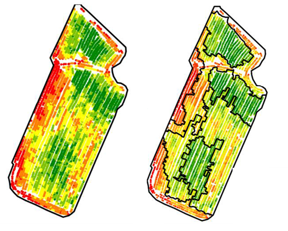
Figure 1. Yield Map (left) and Associated Zoning (right)
The delimitation of intra-plot zones is not something simple. It might seem surprising at first glance because everyone is able, by looking at a colored map, to distinguish large units or large areas on a plot (Figure 1). But in reality, what are we basing this on? On color differences? Differences in shape? On gradients that we have the impression to glimpse? In the end, could not our eyes be a little fooled by the colors displayed on the map, and therefore by the method of colorization applied (this is also a project that it would be interesting to study, notice to amateurs)? Is the variability that we observe within the plot significant or in other words, do the areas that I see and that I can draw manually make sense from an agronomic point of view, and can they be worked on from an operational point of view? What is a zone after all, if not some kind of inert form in the plot? How should a zone be different from its neighbors? When you start to push things a bit further, you might even get into philosophical debates!
Classical zoning
Now let’s move on to the technical side because, computer-wise, the construction of these within-field zones is slightly more complicated than visually. I had already spoken briefly about this in a previous blog post, but we can distinguish two main typologies of methods for making these zoning maps: classification approaches, and segmentation approaches.
Classification methods (mainly equal intervals, quantiles, jenks, or k-means; there are others) are powerful for separating values into different classes. These approaches are often used because they are relatively easy to implement and parameterize (with a number of classes to be filled in, for example). Even so, if you use them, it is clear that these approaches often generate fragmented zone – a kind of pepper and salt effect – because they do not take into account the spatial relationships in the data (this is what you can see on the left map in Figure 1, the data is colored so that you can see something, so it has been classified). The classification is indeed carried out on the attribute values and not on the position of the data in space. There are several ways to get out of this embarrassment. The most common way is to smooth the data (before or after classification) to limit the salt and pepper effect. This smoothing can be done by interpolation if the data are punctual observations (soil or yield data for example) or by using different filters (average, median or other filters) if the data are in the form of rasters. This post-processing is interesting because it allows to arrive at a cleaner map from an operational point of view but it is not always easy to automatically arrive at a suitable map simply because the filter level will also depend on the input data. So we often end up with maps that are sometimes too filtered, sometimes not filtered enough, if the filter parameters are the same. A second way out is to perform a classification taking into account not only the attribute value of the data but also the position of the data in space. The major disadvantage here is that it is not easy to choose the weight to be given to each of these variables (X position, Y position, attribute). Generally speaking, we can generate zoning maps by with classification methods, but these are not methods made at the base for zoning. And let’s add to this that whatever the data, it will always be possible to classify it, even if there is very little variability. In other words, when you’re looking for variability, you always find it…
Segmentation approaches are better suited to spatial data zoning. These methods often come from the field of image processing where one seeks to delimit relatively well-defined shapes. You may have already seen the beautiful Lena on one of the reference images in image processing, the objective being to discriminate each element of the image (Figure 2). Not obvious between the hat, the feathers, the hair or the face.

Figure 2. Lena, a reference in image processing
The problem, as you may have understood, is that a zone in precision agriculture is not something very well defined… but at least we can draw inspiration from what is proposed in the image processing literature to do zoning. There are a lot of different approaches, including :
- region growing methods (you put some sort of seeds or starting points all over a plot and you grow these structures interatively until you get zones – a bit like an oil stain spreading),
- methods that are more oriented towards cutting up images like the “quadtree” approach (where, conversely, the plot is cut up into a lot of small paving stones of different sizes until zones are defined), or
- methods based on contour search (in this case, the boundaries between zones are searched for, and the zones are thus found indirectly)
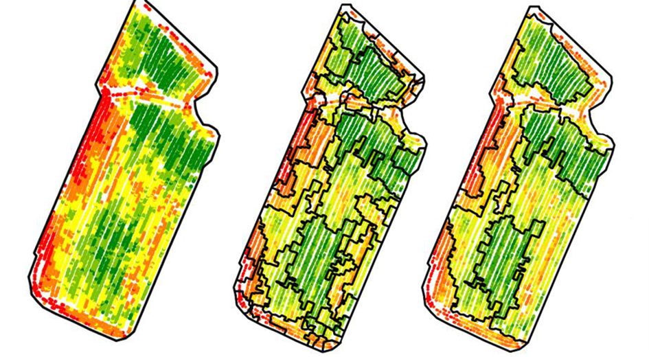
Figure 3. Example of a zoning approach. Zoning after growth of regions (middle) then merging of zones (right)
These approaches regularly generate quite a few zones, and it is often necessary to partially merge the constructed zones to achieve a more operational result with fewer zones (Figure 3).
In contrast to classification approaches, segmentation approaches tend to produce spatial units that are easier to manage and that are less fragmented (less pepper and salt effect) because the spatial location of each observation as well as the spatial neighborhood relationships between each observation are considered (Figure 3). However, these approaches are somewhat more complex to implement and parameterize than classification approaches. For those who are interested, I invite you to have a look at one of my thesis papers and the associated references.
A few additional elements! Zoning can be applied to any type of data, from point data to rasterized data. The approaches are slightly different since when working with raster data, one can directly apply approaches derived from image processing. With point data, one must either go through a preliminary interpolation step (to obtain a raster), or develop a specific approach for point data (this is what we proposed in my thesis). Alongside this, I have so far presented univariate zoning, i.e. one seeks to construct zones on a given attribute (for example, a yield map). But nothing prevents the implementation of multivariate zoning procedures, considering several attributes at the same time (zoning based on both a soil and yield map) or the same attribute over time (zoning based on a history of yield maps) [Figure 4].
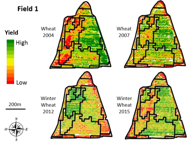
Figure 4. Multi-temporal zoning of performance data
I would also like to emphasize the difference between a class and a zone (Figure 5). You can tell me that these are a little too theoretical considerations, but I still consider that words are important, and this explains, among other things, what we observe with classification or segmentation methods. A zone is a contiguous and closed entity. A class is a label, it is the attribute value of a zone. It is therefore possible to have several zones with the same class. This is important to consider because this is why classification approaches tend to generate a pepper and salt effect. Classification approaches do not create zones directly, they do so indirectly in reality. (Figure 5). It should therefore be said that those who use classification methods construct within-field classes, rather than within-field zones.
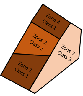
Figure 5. The difference between a zone and a class
After these few general notions, I wanted to introduce some concepts to go a little further into zoning. These are not completely operational approaches, but they could be ideas to dig into. Here we will discuss fuzzy logic and constraint programming, and apply them to zoning!
Fuzzy zoning
This section is a popularized summary of a scientific paper we proposed at the European Precision Agriculture Conference in 2019.
When delimiting intra-plot zones in precision agriculture, we would like these zones to be as different as possible from their neighbors, so that each zone is the place of a differentiated action. However, in agriculture, it is still quite rare to observe very sharp edges in the plots. In reality, it all depends on the agronomic and/or pedological parameters that are studied. One can of course have soil veins, soil units, or extremely different pedogenesis conditions within a plot. But when we look at attributes of vegetation (vigor, biomass, yield…), or topography (altitude, slope…), we will still often have to deal with gradients, major trends that are not so clear-cut. And to convince you of this, you can quickly perform tests with colleagues. Take a high-resolution map (a vegetation or yield map for example), and ask several of your colleagues to delineate 4-5 zones within it. You’ll realize that no one will do exactly the same. Of course, the center or core of the zones will be well identified (perhaps less so if your colleagues are color blind, but that’s another debate), but the borders of the zones will be more or less different. In precision farming, the boundaries between zones are therefore rather blurred. Observations close to the boundaries of each zone could therefore belong to more than one zone, depending on what you want to do with those zones. Depending on a particular operator or farming operation, the objective within the plot will not be the same, so there is no reason for these zones to be identical.
Let’s take the example of the plot below, where the yield observations are displayed (Figure 6). Zones have been pre-delimited with a region growing algorithm (the one in the zoning article of my thesis cited above).
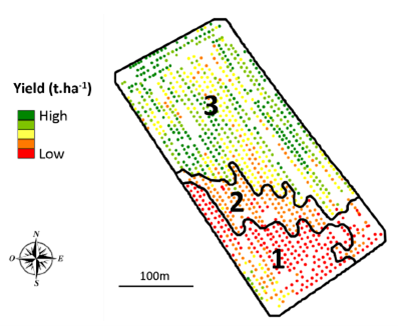
Figure 6. Zoning of a yield map.
The algorithm used led to the creation of 3 zones within the plot. We realize that the yield is relatively high on the north of the plot, average on the east/west diagonal and quite low on the south of the plot. Zone 2 even seems to be a transition zone between zone 1 and zone 3, more than a zone in itself. We also see that in zone 3, the observations in the center of the plot and close to zone 2 are displayed in yellow and one may wonder why these observations could not also belong to zone 2. There is also a yield zone that looks moderately strong southwest of zone 1 but this small entity was not delineated by the region growing algorithm used (this location was probably considered too small by the algorithm to be delineated as a zone, so let’s not consider it).
To visualize this notion of membership of each observation to a zone, we have randomly selected one observation within each zone, and we have relaunched the region growing algorithm (iterative growth from one observation to the next, a bit like an oil stain). With 3 observations at the beginning (1 observation per zone), the final rendering was necessarily composed of 3 zones. And we relaunched this approach 100 times. So we obtained 100 different zonings, and we counted the number of times each observation belonged to the same zone as the one of the 3 initial observations. The map of membership degree (from 0 to 1 – these are percentages) of each observation to a zone is shown in Figure 7.
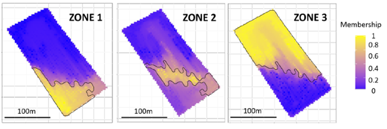
Figure 7. Degree to which each observation belongs to a zone
Within this map, we can clearly see the core of each zone. These are the places that are very marked in yellow, i.e. the places for which the observations are always in the same zone no matter what happens. For example, for zone 1, these are the observations to the southwest of the plot. For zone 3, these are the observations to the north. Conversely, the locations that are very marked in blue are those for which the observations never belong to the zone. The observations to the south of the plot, for example, never belong to zone 3. And then there is everything in between! For example, one realizes how small the core of zone 2 is, but the extent can be large (from a terminological point of view, one differentiates between the “core” or kernel of the zone and its “support” or extent). For this zone 2, there are quite a few cases where observations from zone 1 or 3 may also belong to zone 2. The supports in zones 1 and 3 are smaller. In other words, zones 1 and 3 are well defined and relatively clear, unlike zone 2 (although this was suspected because this zone looks a lot like a transition zone between Zones 1 and 3).
What to do with this map of membership degree? Well, why not look at specific case studies to see to what extent some zoning might be more appropriate than others. Let’s take case n°1 where we will consider that the farmer is subject to strong environmental constraints and cannot accept any risk of overdosing. In this case n°1, the zones must be limited to their core. In case n°2, the farmer uses a low-cost fertilizer whose environmental risks or impact on yield are limited. The zones can therefore be extended to their support. By considering these two cases, and setting thresholds for the membership degree, application maps can be constructed for each zone (Figure 8). Whether for Zone 1 or Zone 3, one realizes how the contour of these zones can change depending on the use case considered. Let’s take the example of zone 3 (on the bottom line of Figure 8). A membership degree greater than 0.3 is considered to represent casst study n°2 because an observation belongs to zone 3 if, in at least 30% of cases, the observation is associated with zone 3 (the support or extent of the zone is therefore large). Conversely, a membership degree greater than 0.7 is considered to represent case study n°1 because it takes at least 70% of cases where the observation is associated with zone 3 for it to be considered to belong there (the support of the zone is therefore smaller; we are getting closer to its core). The same reasoning can be applied for zone 1
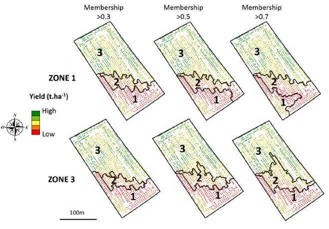
Figure 8. Adapting zoning to use cases.
These results obviously depend on the initial zoning (Figure 6), or on the membership thresholds set, but this work highlights the notion of fuziness associated with within-field zoning, and suggests a way of taking it into account. If it gives you ideas or if it inspires you, do not hesitate to share comments!
Constrained zoning
This section is a popularized summary of a scientific paper we proposed at the European Precision Agriculture Conference in 2021.
When delineating within-field zones in precision agriculture, one has to define what one is trying to achieve. Globally, we are looking for zones that best represent the variability of the plot, i.e. areas that are as homogeneous as possible and as different from their neighbors as possible. That’s good enough, but once we’ve said that, we’re not very advanced either:
- On what do we judge the homogeneity of a zone? On its variance? On the sum of squared differences between each observation and the average of the zone?
- On what do we judge the difference between two neighboring zones? On the average difference between the two zones? On the maximum difference between two observations, each belonging to a zone? On the difference between zones, observation by observation?
- And then, regarding the zones themselves, do we want a specific number of zones on the final map? Do we want zones that have a minimum size? Do we want zones sufficiently geometrical so that they can be handled operationally?
In short, that’s a lot of questions and we can start to see the limits of classification or zoning approaches. Already because we realize that given the number of questions we can ask ourselves here, there is little chance that the relatively simple parameterization of these approaches will satisfy us. And also because in many cases, we find ourselves adding several successive steps (post-processing) to our processing chain to meet all these requests (for example, we remove areas that are too small). By doing so, we have the impression that we are not taking the problem at its root, but rather acting like a fireman by adding steps as soon as there is a problem. And this is not the only limitation of these approaches. For those of you who will be interested in the region growing and merging approach for zoning that I proposed in my thesis (Figure 3), you will realize that merging zones follows an iterative process. Zones are merged progressively by maximizing an operational criterion (which takes into account the attribute distance between each observation and the zone to which it belongs and which also accounts for the geometry of the zones; I invite you to look into this a little more if you are interested). The main limitation being that once a zone is merged, there is no going back. So you potentially end up with a zoned map that is more of a local optimum than a global optimum. That is, each time a zone is merged, the next merge is the one that maximizes the new operational criterion; we see here that it is not a global optimization of the zoning, but an optimization at each iteration, which is not exactly the same thing. Indeed, nothing tells us that a better zoning map could not have been obtained by starting from a fusion that was a little less good at the beginning. This is the limit of incremental approaches. And that’s without taking into account the fact that the merging of zones only takes into account this operational criterion. If you wanted a specific number of zones, you would have to merge always by maximizing this operational criterion but stopping the merging when you get the desired number of zones.
One way to get out of this mess is to look at constraint programming. As its name suggests, we put constraints on our algorithm and force it to find us an optimal solution that meets the constraints set. To do so, we need to define an optimization function (i.e. what the algorithm will try to optimize) and a set of constraints that the algorithm will have to take into account.
So let’s apply this to data zoning! We will start from a zoning obtained from a region growing approach (Figure 9) and we will try to merge the obtained zones (which are too numerous) using a constraint programming method.
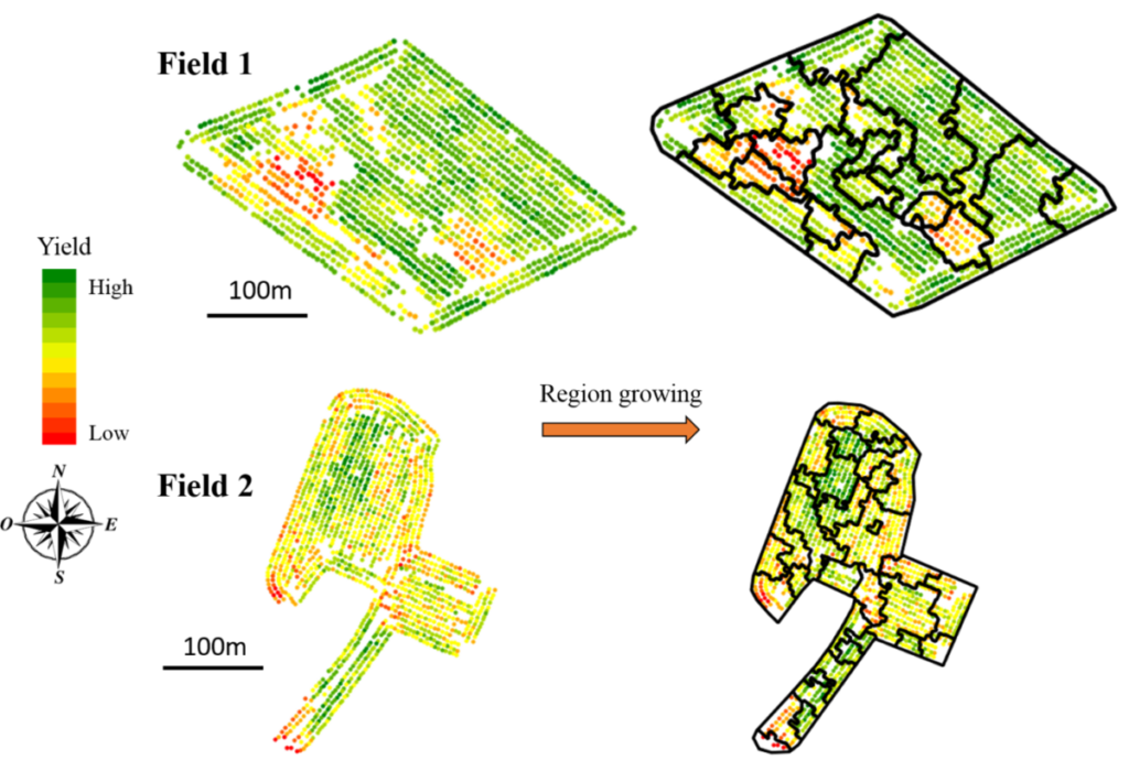
Figure 9. Point yield maps and associated zoning (from a region growth algorithm).
I allow myself here to present the method in the form of notations and equations because I think it is a fairly readable form. If you are not comfortable with the equations, the text should be enough for you to understand the constraints and the optimization function implemented.
The main objective of the constrained fusion algorithm is to generate a set of k final zones Z_i (i \in [1:k]; k \leq N) within the plot (N is the number of initial zones).
Let us start with some notations:
- Each initial zone S_j resulting from the region growth algorithm consists of several spatial observations (make the difference between the initial zones S_j and the final zones Z_i). Each of the observations p in S_j has a yield value called A(p)
- The contiguity between the spatial units S_j is described by the graph G = (V,E)
- For each spatial unit S_j
- area(S_j) is the area of S_j
- card(S_j) is the number of observations in S_j
- \mu(S_j) is the average yield value of the points belonging to S_j
\mu(S_j)=\frac{1}{card(S_j}\sum_{p \in S_j} A(p)
- And
- SSE(S_j) is the sum of squared errors within S_j
SSE(S_j)=\sum_{p \in S_j} (A(p)-\mu(S_j))^2
The constraints of the algorithm :
Now that the notations are clarified, let’s move on to the constraints! To have zones that are consistent with operational constraints in the field, we will consider here that the final zones Z_i must be large enough (threshold \alpha) and that two neighbouing/adjacent zones must have significantly different yield values so that these zones can receive different applications (threshold \beta). The two parameters \alpha and \beta are considered as expert thresholds and appear in constraints n°3 and n°5
- Constraint n°1 : The final zones Z_i cannot be empty
\forall i \in \{1:k\}, Z_i \ne \emptyset
- Constraint n°2 : The final zones Z_i are disjointed (each one is well separated from the others) and each initial zone S_j belongs to one of the final zones Z_i (this is rather logical because the zones Z_i are the result of the merging of the initial zones S_j
\{Z_i\}_{(i \in 1...k)} is a partition of \{1...N\}
- Constraint n°3 : The area of the final zones Z_i must be greather than the threshold \alpha
\forall i \in \{1:k\}, \sum_{S_j \in Z_i} area(S_j) \geq \alpha
- Constraint n°4 : All the initial zones S_j that belong to the same final zone Z_i must be connected to each other. The graph G induced by each zone Z_i is therefore also connected (this constraint is a bit like constraint n°2 to make sure that a final zone is made up of neighboring initial zones, otherwise it would not make sense)
\forall i \in \{1:k\}, G[Z_i] is connected
- Constraint n°5 : The difference in yield between two neighboring zones must be greater than the threshold \beta
\forall i1,i2 \in \{1:k\}, i1 \ne i2, Z_1 ADJ Z_2 \Rightarrow \vert \mu({Z_i}_1) - \mu({Z_i}_2) \vert \geq \beta
With ADJ the relation of adjacency :
Z_1 ADJ Z_2 \Leftrightarrow \exists {S_j}_1 \in Z_1, \exists {S_j}_2 \in Z_2 such as (j_1,j_2) \in E
The optimization function of the algorithm :
The constraint programming approach aims at optimally merging the initial zones in order to minimize the function \f which is the sum of the squared differences between the yield of each observation and the average yield of the zone to which the observation belongs :
f = \sum_{i \in 1...k} SSE(S_j) = \sum_{i \in 1...k} \sum_{p \in U_(S_j \in Z_i)} (A(p) - \mu(Z_i))^2
For the tests that we carried out, we chose to set the thresholds \alpha and \beta respectively at 0.5 ha (minimum area of zones) and 1 ton per ha (minimum difference in yield between neighboring zones). To run constraint programming algorithms, it is generally necessary to use a solver that already contains optimization modules and is able to take constraints into account. It is not very simple to run a constraint programming algorithm on languages such as R or Python. In our case, we used a solver named “Choco”, which seemed to be rather adapted to our problem.
The results of constraint optimization are shown in figures 10 and 11. It is interesting to note that the algorithm is not always able to find solutions to the constraints we set for it. This is not bad! This means, for example, that for Field 2, we cannot find a zoning for more than 4 zones that respect our constraints of a minimum surface area of 0.5 ha and a minimum yield difference of 1 tonne per ha. When we have these results available, there are several ways to consider them. Either we want to work with a particular number of zones and therefore we select the corresponding zoning. Either one looks for the result with the lowest value of the function f (since one has tried to minimize f for each number of zones in the plot), regardless of the number of zones. In the case of Field 1, for example, the function f reaches a minimum for 5 zones before rising sharply enough for 6 zones. We have not compared these results here with those of a more conventional zoning method (but it is already known that the conventional method would have given results regardless of the number of zones required)
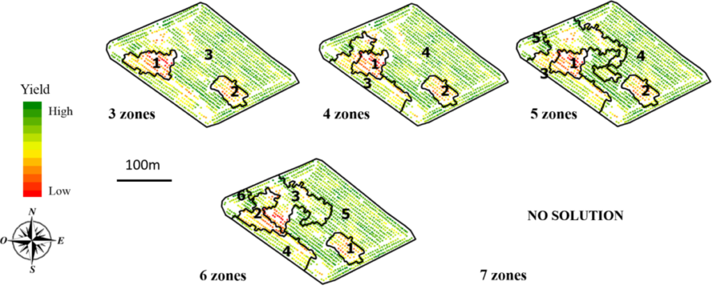
Figure 10. Optimization under constraints (Plot 1) between 3 and 7 zones.
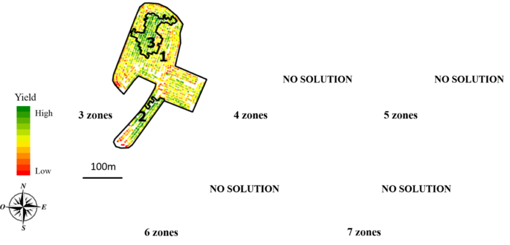
Figure 11. Optimization under constraints (Plot 2) between 3 and 7 zones.
In this small case study, we only set constraints on the size of the zones and the attribute difference between two neighbouring zones (constraints 1, 2 and 4 are rather associated with the zoning problem in general and should therefore always be kept). Other constraints could have been considered, for example on the shape of the zones, or on the maximum variability within each zone. Anything is possible. However, it is necessary to ensure that the constraints make sense from an agronomic and operational point of view. Note also that constraint programming is interesting, but it necessarily takes more time than more traditional zoning approaches. The solver helps speed up and improve the search for optimal solutions, but it takes time since constraints must be taken into account. And the more constraints there are, the longer the search time can be.
Within-field zoning raises a number of important questions when you start to look at it a little bit. Between fairly blurred zone boundaries, operational constraints to be integrated, or the possibility of working in the uni or multivariate space, the subject is far from being fully addressed. Keep in mind, however, that much of this work remains exploratory (notably the sections on fuzzy zoning and constrained zoning). Their implementation and industrialization remains quite possible. However, it must be relevant to the profession, it must provide real added value compared to conventional approaches, and it must not make the analysis of within-field zones even more complex than it is at present
Support Aspexit’s blog posts on TIPEEE
A small donation to continue to offer quality content and to always share and popularize knowledge =) ?