
Dans le post précédent, on a dressé un portrait assez général des capteurs de rendement et des données associées. On revient ici sur une question récurrente en rapport avec les données de rendement : Comment s’assurer que les données de rendement soient assez fiables pour pouvoir les utiliser correctement ? Nous allons donc passer en revue les principales sources d’incertitude de ces jeux de données ; et évoquer certaines des méthodes qui ont été proposées pour s’attaquer à ce problème. Nous ne détaillerons pas l’ensemble de ces méthodes, ce serait beaucoup trop fastidieux mais la bibliographie reste à disposition pour les intéressés !
Pourquoi filtrer ses cartes de rendement ?
Les cartes de rendement ont été largement reconnues comme une source d’information précieuse pour la prise de décisions sur le terrain (Diker et al. 2004 ; Florin et al. 2009 ; Pringle et al. 2003). Elles fournissent effectivement un aperçu global de la variabilité spatiale sur le terrain, ce qui les rendent intéressantes pour cibler des zones d’intérêt dans les parcelles ou des secteurs sur lesquels il pourrait être pertinent de réaliser des applications modulées. Comme on l’a vu dans le post précédent, des centaines voire des milliers d’observations spatiales de rendement sont générées et sont prêtes à être utilisées dans le processus décisionnel. Bien que ce volume considérable de données soit essentiel pour la gestion et la prise de décision sur le terrain, ces jeux de données doivent être utilisés avec un peu de prudence et de recul.
Ces jeux de données contiennent en effet beaucoup d’observations défectueuses ou d’erreurs techniques qu’il faut éliminer pour assurer la qualité des données (Arslan et Colvin, 2002 ; Blackmore et Moore, 1999). Il faut bien comprendre que considérer ces observations défectueuses comme des « erreurs » est en fait un peu faux. Ce sont plutôt des observations qui ne correspondent pas au véritable rendement observé sur les parcelles et qu’on aurait pu attendre de l’itinéraire cultural. Si on voulait être précis, il faudrait dire que c’est le processus d’acquisition des données (avec un capteur embarqué sur la moissonneuse-batteuse, laquelle récolte la parcelle) qui conduit à générer des données qui, parfois, ne sont pas cohérentes avec la réalité. Ce n’est pas le capteur en lui-même qui fait une erreur (même si ça peut arriver) mais c’est le fait d’avoir un système embarqué qui conditionne la façon d’acquérir les données. Vous devriez y voir un peu plus clair par la suite. Dans la suite de ce post, je parlerai « d’erreurs de rendement » parce que c’est plus simple mais vous aurez compris (je l’espère) que c’est une simplification de la réalité.
Au vu des erreurs de rendement, ces jeux de données de rendement sont souvent sévèrement filtrés pour s’assurer que les analyses ultérieures ne soient pas défectueuses (Robinson et Metternicht, 2005 ; Sudduth et Dummond, 2007 ; Sun et al. 2013). Plusieurs auteurs ont montré à quel point une carte de rendement pouvait évoluer avant et après avoir supprimé les observations jugées anormales (Simbahan et al., 2004 ; Sudduth et Dummond, 2007). Griffin et al. (2008) ont même montré que ces dernières observations pouvaient influencer les décisions de gestion au champ. Attention quand même parce que l’article de Griffin et al. (2008) reste assez qualitatif. Il n’existe pas vraiment d’études qui ont étudié vraiment très en profondeur l’impact que pouvaient avoir les observations défectueuses sur la cartographie de rendement. Si ça ne tenait qu’à moi, j’aurais tendance à dire que tout dépend ce qu’on veut faire des données de rendement. Si l’on souhaite avoir une information de rendement moyenne à la parcelle ou dégager des grosses tendances de rendement dans les parcelles, une méthode de filtrage assez simple devrait suffire et rendre des résultats assez concluants. Si l’on souhaite par contre rentrer dans le détail, par exemple en cherchant à valider des résultats d’expérimentation, ou à moduler des apports de façon précise, il faudrait mieux travailler avec des méthodes un peu plus avancées et un peu plus robustes. Il ne faut par contre jamais considérer que le nettoyage des données sera parfait ! L’expertise du terrain, que ce soit celle de l’agriculteur, de son conseiller ou d’un chef d’expérimentation, qui connait la parcelle, est primordiale.
Typologies d’erreurs dans les cartes de rendement
Ces erreurs techniques ou ces observations défectueuses ont été largement documentées dans la littérature. Lyle et ses collaborateurs (2013) ont proposé une catégorisation de ces erreurs en quatre grands groupes : (i) la dynamique de récolte de la moissonneuse-batteuse, (ii) les mesures continues du rendement et de l’humidité, (iii) la précision du système de positionnement et (iv) l’opérateur de la moissonneuse-batteuse. Ces erreurs techniques sont brièvement décrites ici avec certaines des méthodologies qui ont été proposées par la communauté scientifique pour identifier ces observations défectueuses.
- La dynamique de la récolte de la machine comprend trois décalages différents, appelés temps de latence, temps de montée en charge et temps de descente en charge (Blackmore et Moore, 1999). Le temps de latence induit un décalage entre l’emplacement actuel et l’emplacement réel d’une observation de rendement dans l’espace parce que le rendement n’est pas mesuré au moment où la plante est coupée (c’est en quelque sorte le temps entre le moment où la plante est coupée et le moment où le grain arrive jusqu’au capteur de rendement). Plusieurs méthodes ont été mises au point pour déterminer ce décalage, soit par (i) des méthodes géostatistiques (Chung et al., 2002), (ii) des techniques de traitement d’images (Lee et al. 2012) et (iii) des méthodes de déconvolution du signal (Arslan, 2008 ; Reinke et al. 2011). Le temps de montée en charge, à l’entrée de parcelle lors d’une nouvelle ligne de récolte, conduit à une sous-estimation du rendement car le flux de grains dans la moissonneuse augmente petit à petit et n’a pas encore atteint un plateau, c’est-à-dire le régime permanent. Par conséquent, les mesures de rendement ne correspondent pas aux valeurs réelles de rendement attendues. A la fin d’une ligne de récolte, il se peut qu’une partie du grain continue à circuler dans la moissonneuse même s’il n’y a plus de plantes à récolter et que le temps de latence ait été atteint. Par conséquent, les dernières observations d’une ligne de récolte sont généralement sous-estimées. Les méthodes qui ont été proposées jusqu’à présent sont exclusivement visuelles, c’est-à-dire que le flux de grain est tracé en fonction du temps de parcours dans la parcelle ou de la distance d’avancement de la machine, et que les données situées avant ou après le plateau de rendement sont supprimées (Lyle et al. 2013 ; Simbahan et al. 2004).
- Les mesures continues se rapportent aux erreurs dans les observations de rendement et d’humidité dus à des mal fonctionnements de capteurs. Jusqu’à présent, les travaux de recherche ont cherché à trouver des seuils, déterminés pour la plupart de façon empirique, afin de déterminer ces types d’erreurs (Sudduth et Drummond, 2007 ; Taylor et al. 2007). Arslan et Colvin (2002) ont par exemple mis en avant des précisions de capteurs variant de 1 et 4 %, tandis que d’autres auteurs ont constaté des différences allant jusqu’à 10 % selon les conditions environnementales pendant l’acquisition des données, p. ex. des pentes raides (Reitz et Kutzback, 1996). Pour surmonter ce problème, quelques études ont porté sur l’impact des vibrations de la moissonneuse-batteuse sur la précision de la mesure du rendement (Hu et al. 2012 ; Jingtao et Shuhui, 2010).
- La précision des systèmes de positionnement peut conduire (i) à des observations en dehors des limites de la parcelle, (ii) à plusieurs observations de rendement à la même position dans l’espace, c’est-à-dire à des points colocalisés, ou (iii) à des écarts dans l’espace par rapport à la ligne de récolte (Blackmore et Moore, 1999). Les deux premiers types d’erreurs peuvent être facilement traités en éliminant les points situés à l’extérieur des limites parcellaires ou les points dont les coordonnées sont similaires (Robinson et Metternicht, 2005 ; Simbahan et al. 2004). Certains algorithmes ont été développés pour reconstruire précisément les lignes de récolte en étudiant les angles formés par des points de mesure consécutifs (Lyle et al., 2013). Les points suspects – ceux par lesquels la moissonneuse-batteuse a peu de chance d’être passés – sont retirés du jeu de données.
- Le dernier type d’erreurs concerne l’opérateur de la moissonneuse-batteuse. Premièrement, de grandes variations de vitesse sont susceptibles d’avoir un impact important sur la qualité de l’ensemble des données de rendement (Arslan et Colvin, 2002 ; Sudduth et Drumond, 2007). Les questions de vitesse sont généralement traitées de la même façon que les questions de mesures continues de rendement et d’humidité, c’est-à-dire en fixant des seuils globaux pour l’ensemble du jeu de données ou des seuils locaux seulement pour des données voisines dans l’espace (Lyle et al., 2013). Il peut aussi arriver que l’opérateur, en conduisant, chevauche des lignes de récolte déjà en partie ou totalement récoltées, ce qui est susceptible d’entraîner des observations de rendement aberrantes. Certains auteurs ont mis l’accent sur cet effet de » barre de coupe partiellement utilisée » et ont proposé des méthodes de prétraitement vectoriel pour tenir compte de ces chevauchements, principalement en reconstruisant le passage de la machine dans la parcelle (Drummond et al., 1999). Ces méthodes vectorielles dépendent fortement de la précision du positionnement du dispositif GNSS et nécessitent un temps de traitement important. D’autres auteurs ont proposé des systèmes embarqués spécifiques, notamment des capteurs ultrasoniques (Zhao et al., 2010). Enfin, les tournières sont également à l’origine de mauvaises estimations de rendement (Lyle et al. 2013). Les études consacrées à ces dernières sources d’erreurs – bien que limitées dans la littérature – se sont concentrées sur la recherche des points à l’intérieur des tournières en utilisant des mesures de distance ou d’angle entre des observations consécutives. Les points suspects sont éliminés.
Des exemples de ces typologies d’erreurs sont présentés sur les deux figures suivantes:
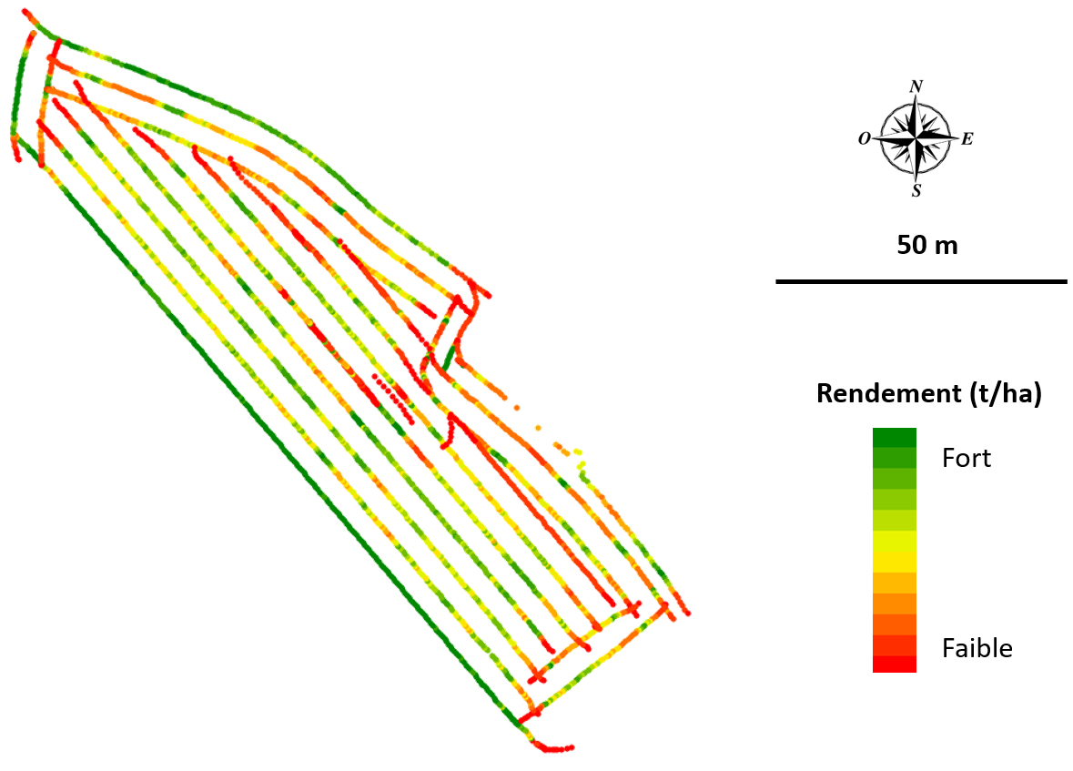
Figure 1. Carte de rendement
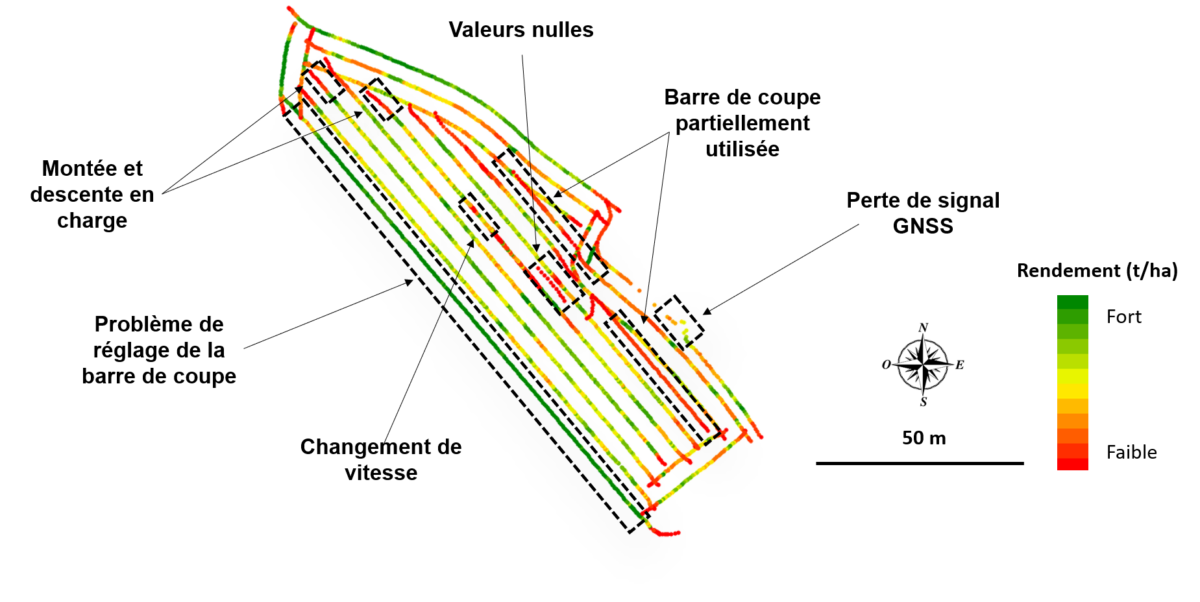 Figure 2. Carte de rendement avec sources d’erreurs labellisées.
Les capteurs embarqués comme les capteurs de rendement génèrent une quantité d’observations très importante. Au vu du volume considérable d’observations et du besoin de travailler de façon opérationnelle avec ces données, les approches de filtrage se doivent d’être à la fois automatisées, très générales et non paramétriques – c’est-à-dire qu’on ne doit pas avoir à régler plein de paramètres tout le temps (Simbahan et al. 2004 ; Spekken et al. 2013). La condition d’automatisation est très importante, notamment parce que le nombre de données de rendement à traiter ira en augmentant. L’automatisation ne veut néanmoins pas dire que l’expertise humaine peut être mise de côté, bien au contraire. C’est l’expert qui jugera, au vu de la méthode utilisée et de ses connaissances sur la parcelle, si le traitement lui convient. Les méthodes de filtrage générales et non paramétriques sont également à privilégier en raison de la diversité des jeux de données à traiter. Ces jeux de données sont effectivement acquis avec des systèmes d’acquisition différents – machines, capteurs – et sur des cultures variées, avec différents opérateurs et dans des conditions d’acquisition variables (topographie, climat…). Il est donc important de s’assurer que les approches sont capables de fournir des résultats concluants quel que soit le jeu de données à analyser. Même si de nouvelles solutions techniques existent pour améliorer la qualité des jeux de données de rendement, par exemple les capteurs à ultrasons (Zhao et al. 2010), les moissonneuses-batteuses actuelles sont loin d’en être toutes équipées (il resterait à vérifier si ces capteurs à ultrasons fonctionnent bien en condition opérationnelles). Des méthodes générales sont donc nécessaires pour traiter les jeux de données provenant de plusieurs types de machines, quel que soit le niveau d’équipement supplémentaire installé.
Il faut garder à l’esprit que les jeux de données de rendement seront potentiellement utilisés pour prendre une décision opérationnelle, ou comme point d’entrée de modèles agronomiques. Les méthodes de filtrage des données doivent donc être suffisamment robustes pour que le processus de prise de décision soit précis et sans faille. Une des limites de la littérature actuelle est que la plupart des approches existantes sont semi-automatiques et reposent presque exclusivement sur des seuils et des filtres d’experts. La conséquence principale étant que le traitement des cartes de rendement à grande échelle (mais même au niveau d’une exploitation entre plusieurs années par exemple), soit rendus compliqués parce que les paramètres de filtrage peuvent être influencés par chaque producteur de cartes et des opérateurs qualifiés pourraient être nécessaires pendant une période de temps considérable (Spekken et al. 2013). Encore une fois, l’utilisateur final aura la main sur le traitement issu d’une méthode automatisé, et pourra considérer que le traitement lui parait pertinent ou non. Pour les lecteurs intéressés, une méthode de filtrage tentant de répondre au maximum à ces contraintes a été proposée dans le cadre de ma thèse (Leroux et al., 2018).
Quelques éléments complémentaires
Jusqu’ici, nous nous sommes concentrés sur différentes erreurs de rendement, mais en faisant l’hypothèse que les informations de rendement collectées sont quand même majoritairement de qualité (sinon, si tout était mauvais, comment pourrait-on considérer que des données sont à enlever et d’autres à garder). C’est-à-dire que nous avons fait l’hypothèse qu’au départ, le capteur de rendement était bien étalonné…. L’étalonnage du capteur de rendement (et d’humidité…) est très important pour être sûr que les valeurs de rendement obtenues puissent être utilisées telles quelles, c’est-à-dire en valeur absolue. Si le capteur est mal étalonné, rien ne nous dit que les valeurs sont celles attendues ; par contre on peut quand même faire l’hypothèse que le capteur n’inversera pas les tendances de rendement observées (en d’autres termes qu’il ne va pas considérer qu’un rendement faible est fort et inversement). Tout ça pour dire que même mal étalonné, un capteur de rendement devrait quand même assez fidèlement reproduire les grandes tendances de rendement dans la parcelle, même si ces valeurs peuvent être fausses en absolu. De façon optimale, il faudrait pouvoir étalonner le capteur tous les jours (au vu du changement des conditions d’acquisition, comme l’humidité par exemple) et quand le type de plantes récoltées change. C’est malheureusement difficilement envisageable d’un point de vue opérationnel ; mais l’étalonnage du capteur de rendement devrait être fait au moins correctement une fois au début de la saison de récolte. On pourrait également imaginer corriger la carte de rendement en absolu à partir d’une valeur de rendement de référence à la parcelle, par exemple celle obtenue à la pesée en sortie de parcelle (si tant est que la pesée soit faite pour chaque parcelle). Cela pourrait être le moyen de comparer le rendement moyen « vrai » à la parcelle et le rendement moyen obtenu avec les données de rendement. Attention néanmoins à l’erreur d’étalonnage qui n’est pas forcément linéaire sur toute la plage de valeurs de rendement (c’est-à-dire que l’erreur de rendement sera peut-être plus importante pour des valeurs de rendement fortes que pour des valeurs de rendement faibles). Attention également au fait qu’en corrigeant avec une valeur moyenne, on ne prend pas en compte la variance du rendement que l’on pourrait attendre dans la parcelle.
La majorité des cartes de rendement sont présentées sous la forme de données ponctuelles (de points). Il faut néanmoins garder à l’esprit que l’information de rendement est en réalité une surface, celle donnée par la vitesse d’avancement de la moissonneuse et sa barre de coupe. Rajoutons à cela, si l’on veut être tatillon, qu’au moment où les plantes sont coupées, ce sont les plantes au centre de la barre de coupe qui sont ramenées en premier dans la moissonneuse, par rapport aux plantes aux extrémités de la barre de coupe. Tout cela pouvant jouer sur la pondération réelle à donner aux observations de rendement. Rentrer dans ces considérations devient extrêmement complexe et on pourrait questionner la pertinence d’aller dans tant de détail. Certains travaux de recherche sont quand même allés jusqu’à la modélisation du fonctionnement d’une moissonneuse batteuse pour prendre en compte ces aspects-là (Reinke et al., 2011). Comme les moissonneuse-batteuse lsont toutes différentes, cette approche parait malheureusement un peu trop complexe pour être appliquée sur le terrain. Pour terminer, en rapport avec la modélisation du fonctionnement de la moissonneuse-batteuse, j’aimerais revenir sur un point que nous avons un peu laissé de côté jusqu’ici, le retour d’Otons (présenté sur la figure de la moissonneuse batteuse dans le post précédent). Pour comprendre ce phénomène, on peut s’imaginer qu’au temps ‘t’, un stock de grain rentre dans la moissonneuse. Dans un système parfait, tout le stock de grain qui rentre en même temps dans la moissonneuse, arriverait en même temps dans la trémie. Malheureusement, une partie de ce grain (qui n’a pas forcément été bien battu ou tamisé) reste dans les organes de la moissonneuse et est mélangé avec le ou les stocks de grain qui continuent à arriver au temps ‘t+1’ par exemple. Ce phénomène pose donc question quand à la pondération de rendement sur chacun des points de mesure réalisés puisqu’en réalité, le rendement mesuré ne correspond qu’à une partie du grain réellement récolté à un point précis dans l’espace. Peut-on faire l’hypothèse que ce retour d’Otons reste à peu près stable pendant toute la récolte et donc que toutes les observations seraient affectées de la même manière ? Ca pourrait être à vérifier… C’est en tout cas l’hypothèse que nous faisons.
Vous m’excuserez pour les références bibliographiques que je n’ai pas reclassé spécifiquement pour ce post… mais vous devriez pouvoir les retrouver sans problème =)
- Acevedo-Opazo, C., Tisseyre, B., Guillaume, S., & Ojeda, H. (2008). The potential of high spatial resolution information to define within-vineyard zones related to vine water status. Precision Agriculture, 9, 285-302.
- Adams, R., & Bischof, L. (1994). Seeded Region Growing. IEEE Transactions on Pattern Analysis and Machine Intelligence, 16, 641-647
- Akdemir, B. (2016). Evalution of precision farming research and applications in Turkey. VII International Scientific Agriculture Symposium « Agrosym 2016 ». 6-9 October 2016, Jahorina, Bosnia and Herzegovina. Proceedings Book. pp.1498-1504.
- Angiulli, F., Fassetti, F., & Palopoli, L. (2009). Detecting outlying properties of exceptional objects. ACM Transactions on Database Systems, 34, 1, 1-7.
- Angiulli, F., Fassetti, F., & Palopoli, L. (2012). Discoverying characterizations of the behavior of outlier sub -populations. IEEE Transactions on Knowledge and Data Engineering, 25, 1280-1292
- Arslan, S., & Colvin, T. (2002 ). Grain yield mapping : yield sensing, yield reconstruction, and errors. Precision Agriculture, 3, 135-154
- Arslan, S. (2008). A Grain Flow Model to Simulate Grain Yield Sensor Response. Sensors, 8, 952–962.
- Arun, P.V. (2013). A comparative analysis of different DEM interpolation methods. The Egyptian Journal of Remote Sensing and Space Science, 16, 2, 133-139.
- Baluja, J., Diago, M., Goovaerts, P., & Tardaguila, J. (2012 ). Assessment of the spatial variability of anthocyanins in grapes using a fluorescence sensor: relationships with vine vigour and yield. Precision Agriculture, 13, 457–472.
- Bakhsh, A., Jaynes, D.B., Colvin, T.S., & Kanxar, R.S. (2000). Spatio-temporal analysis of yield variability for a corn-soybean field in Iowa. Agricultural and Biosystems Engineering, 43, 31-38.
- Barnaghi, P., Sheth, A., & Henson C. (2013 ) “From data to actionable knowledge: Big data challenges in the web of things,” Intelligent Systems, IEEE, 28, 6–11, 2013.
- Basso, B., Bertocco, M., Sartori, L., & Martin, E.C. (2007 ). Analyzing the effects of climate variability on spatial pattern of yield in a maize–wheat–soybean rotation. European Journal of Agronomy, 26, 82–91.
- Basso, B., Fiorentino, C., Cammarano, D., Cafiero, G., & Dardanelli, J. (2012 ). Analysis of rainfall distribution on spatial and temporal patterns of wheat yield in Mediterranean environment. European Journal of Agronomy, 41, 52-65.
- Basso, B., B. Dumont, D. Cammarano, A. Pezzuolo, F. Marinello, & L. Sartori. (2016 ). Environmental and economic benefits of variable rate nitrogen fertilization in a nitrate vulnerable zone . Science of the Total Environment. 545–546, 227–235
- Bellehumeur, C., Legendre, P., & Marcotte, D. (1997). Variance and spatial scales in a tropical rain forest: changing the size of sampling units. Plant Ecology, 130, 89-98.
- Ben-Gal, I. (2005 ). Outlier Detection. The Data Mining and Knowledge Discovery Handbook: A Complete Guide for Practitioners and Researchers. Boston: Kluwer Academic Publishers.
- Berducat, M., Boffety, D. (2000). Gestion de l’information parcellaire – cartographie du rendement à la récolte. Ingénieries – E A T, IRSTEA édition 2000, p. 53 – p. 62
- Beyer, K., Goldstein, J., Ramakrishnan, R., & Shaft, U. (1999). When is nearest neighbor meaningful ? In Proceedings of the 7 th ICDT, Jerusalem, Israel.
- Bivand R.S., Pebesma, E.J., & Gomez-Rubio, V. (2008). Applied Spatial Data Analysis with R. New York, NY: Springer
- Blackmore, B. S., & Moore, M. (1999). Remedial correction of yield map data. Precision Agriculture, 1, 53 – 66.
- Blackmore, S., Godwin, R.J., & Fountas, S. (2003 ). The analysis of spatial and temporal trends in yield map data over six years. Biosystems Engineering. 84, 455-466.
- Bongiovanni, B. and Lowenberg-Deboer, J. (2004). Precision agriculture and sustainability. Precision Agriculture, 5, 359_387.
- Bongiovanni, R.G., Robledo, C.W., & Lambert, D.M. (2007). Economics of site-specific nitrogen management for protein content in wheat. Computers and Electronics in Agriculture, 58, 13–24.
- Bramley, R.G.V., & Hamilton, R.P. (2004). Understanding variability in winegrape production systems. Australian Journal of Grape and Wine Research, 10, 32–45
- Bramley, R.G., Hill, P.A., Thorburn, P.J., Kroon, F.J., & Panten, K (2008 ). Precision agriculture for improved environmental outcomes: some Australian perspectives. Agriculture Forest Research, 3, 161–178.
- Breunig, M.M., Kriegel, H.P., Ng, R.T., & Sander, J. (2000). Lof: identifying density-based local outliers. In Proceedings of 2000 ACM SIGMOD International Conference on Management of Data. ACM Press, pp. 93 – 104
- Cambardella, C.A., Moorman, T.B., Novak, J.M., Parkin, T.B., Karlen, D.L., Turco, R.F. et al. (1994). Field -scale variability of soil properties in central Iowa soils. Soil Science Society of America Journal, 58, 1501 – 1511.
- Cambardella, C. A., & Karlen, D. L. (1999). Spatial analysis of soil fertility parameters. Precision Agriculture, 1, 5-14.
- Cao, Q., Cui, Z., Chen, X., Khosla, R., Dao, T.H., & Miao, Y. (2012 ). Quantifying spatial variability of indigenous nitrogen management in small scale farming. Precision Agriculture, 13, 45–61.
- Cassman, K. G. (1999 ). Ecological intensification of cereal production systems: yield potential, soil quality, and precision agriculture. Proceedings of the National Academy of Sciences of the United States of America , 96, 5952–5959
- Cerovic, Z.G., Goutouly, J.P., Hilbert, G., Destrac-Irvine, A., Martinon, V., & Moise, N. (2009 ) Mapping winegrape quality attributes using portable fluorescence-based sensors. In: Best S (ed) Progap INIA, FRUTIC 09, Conception, Chile, pp 301–310
- Chen, D., Lu, C-T., Kou, Y. & Chen, F. (2008). On Detecting Spatial Outliers. Geoinformatica, 12, 455-475
- Chung, S. O., Sudduth, K. A., & Drummond, S. T. (2002 ). Determining Yield Monitoring System Delay Time With Geostatistical and Data Segmentation Approaches. Transactions of the ASAE, 45, 915-926.
- Chung, S.O., Choi, M.C., Lee, K.H, Kim, Y.J, Hong, S.J., Li, M. (2016 ). Sensing Technologies for Grain Crop Yield Monitoring Systems: A Review. Journal of Biosystems Engineering, 41, 408-417.
- Cid-Garcia, N.M., Albornoz, V., Rios-Solis, Y.A., & Ortega, R. (2013 ). Rectangular shape management zone delineation using integer linear programming. Computer and Electronics in Agriculture, 93, 1–9.
- Clifford, P., Richardson, S., & Hemon, D. (1989 ). Testing the association between two spatial processes. Biometrics, 45, 123–134.
- Collins, E.D., & Chandrasekaran, K. (2012 ). A Wolf in Sheep’s Clothing? An Analysis of the ‘Sustainable Intensification’ of Agriculture (Friends of the Earth International, Amsterdam, 2012)
- Colvin, T.S., Jaynes, D.B., Karlen, D.L., Laird, D.A., & Ambuel, J.R. (1997 ). Yield variability within a central Iowa field. Transactions of the ASAE, 40, 883–889.
- Comifer (2007 ). Teneur en P, K et Mg des organes végétaux récoltés pour les cultures de plein champ et les principaux fourrages, Comifer, Paris, 6 pages.
- Cox, S. (2002). Information technology : the global key to precision agriculture and sustainability. Computers and Electronics in Agriculture, 36, 93-111.
- Cressie, N. A., (1991). Statistics for Spatial Data. John Wiley & Sons, New York.
- Cressie, N. (1996). Change of support and the modifiable areal unit proble. Geographical Systems, 3, 159 – 180
- Dale, M.R.T, & Fortin, M.J. (2002). Spatial autocorrelation and statistical tests in ecology. Eco Science , 9, 162-167
- Davatgar, N., Neishabouri, M.R., & Sepaskhah, A.R. (2012 ). Delineation of site specific nutrient management zones for a paddy cultivated area based on soil fertility using fuzzy clustering. Geoderma, 173–174, 111–118.
- Debuisson, S., Germain, C., Garcia, O., Panigai, L., Moncomble, D., Le Moigne, et al. (2010 ). Using Multiplex® and Greenseeker™ to manage spatial variation of vine vigor in Champagne. 10th International Conference on Precision Agriculture.
- de Oliveira, R. P., Whelan, B. M., McBratney, A. B., & Taylor, J. A. (2007 ). Yield variability as an index supporting management decisions: YIELDex. Proceedings of the 6th European Conference on Precision Agriculture, 281–288.
- DEFRA (2013). Farm Practices Survey Autumn 2012 – England. Department for Environment, Food and Rural Affairs (DEFRA). 41pp.
- Di Virgilio, N., Monti, A., & Venturi, G. (2007). Spatial variability of switchgrass (Panicum virgatum L.) yield as related to soil parameters in a small field. Field Crops Research, 101, 232-239.
- Diker, K., D.F. Heerman, & M.K. Brodahl. (2004 ). Frequency analysis of yield for delineating yield response zones. Precision Agriculture, 5, 435–444.
- Drummond, S. T., Fraisse, C. W., & Sudduth, K. A. (1999 ). Combine Harvest Area Determination by Vector Processing of GPS Position Data. Transactions of the ASAE, 42, 1221–1227.
- Duan, L., Xu, L., Guo, F., Lee, J., & Yan, B. (2007). A local-density based spatial clustering algorithm with noise. Information Systems, 32, 978–986
- Duan L., Tang, G., Pei, J., Bailey, J., Campbell, A., & Tang, C. (2015 ). Mining outlying aspects on numeric data. Data Mining Knowledge Discovery, 29, 1116–1151
- Dutilleul, P. (1993). Modifying the t-test for assessing the correlation between two spatial processes. Biometrics, 49, 305–314.
- Eghball, B., Power, J.F. (1995). Fractal description of temporal yield variability of 10 crops in the United States. Agronomy Journal, 87, 152-156.
- Ertoz, L., Eilertson, E., Lazarevic, A., Tan, P., Srivastava, J., Kumar, V., & Dokas, P. (2004). The MINDS – Minnesota Intrusion Detection System, in Data Mining, A. Joshi H. Kargupta, K. Sivakumar, and Y. Yesha (Eds.) Next Generation Challenges and Future Directions.
- Ester, M., Kriegel, H.-P., Sander, J., & Xu, X. (1996). A density-based algorithm for discovering clusters in large spatial databases with noise. In E. Simoudis, J. Han, and U. Fayyad (Eds.), Proceedings of Second International Conference on Knowledge Discovery and Data Mining , Palo Alto, CA, USA: AAAI Press, pp 226–231.
- European Parliamentary Research Service (2016 ). Precision Agriculture and the Future of Farming in Europe, STOA, Brussels, European Union.
- EU SCAR. (2012). Agricultural knowledge and innovation systems in transition. Brussels: EU.
- Fairfield Smith, H. (1938). An empirical law describing heterogeneity in the yield of agricultural crops. The Journal of Agricultural Science, 28, 1–23.
- FAO (2017). The future of food and agriculture. http://www.fao.org/3/a-i6644e.pdf (accessed 05/06/2018)
- Fauvel, M., Chanussot, J., & Benediktsson, J.A. (2011). A spatial–spectral kernel-based approach for the classification of remote-sensing images. Pattern Recognition, 45, 381-392.
- Fauvel, M., Tarabalka, Y., Benediktsson, J.A., Chanussot, J., & Tilton, J. (2012). Advances in Spectral-Spatial Classication of Hyperspectral Images. Proceedings of the IEEE, Institute of Electrical and Electronics Engineers, 101, 652-675.
- Filzmoser, P., Ruiz-Gazen, A., & Thomas-Agnan, C. (2014). Identification of local multivariate outliers. Statistical Papers, 55, 29-47.
- Florin, M.J., McBratney, A.B., & Whelan, B.M. (2009 ). Quantification and comparison of wheat yield variation across space and time. European Journal of Agronomy, 30, 212-219.
- Fountas, S., Pedersen, S.M., & Blackmore, S. (2005). ICT in Precision Agriculture – diffusion of technology. In « ICT in Agriculture: Perspectives of Technological Innovation » edited by E. Gelb, A. Offer. 15pp.
- Fraisse, C.W., Sudduth, K.A., Kitchen, N.R. (2001). Delineation of site-specific management zones by unsupervised classification of topographic attributes and soil electrical conductivity. Transactions of the ASAE, 44, 155-166.
- Fulton, J.P., Shearer, S.A., Chabra, G., & Higgins, S.F. (2001 ). Performance assessment and model development of a variable-rate, spinner-disc fertilizer applicator. Transactions of the ASAE, 44, 1071-1081.
- Fulton, J. P., Shearer, S.A., Higgins, S.F., Darr, M.J., & Stombaugh, T.S. (2005 ). Rate response assessment from various granular VRT applicators. Transactions of the ASAE, 48, 2095‐2103.
- Garnett, T., Appleby, M. C., Balmford, A., Bateman, I. J., Benton, T. G., Bloomer, P., et al. (2013 ). Sustainable intensification in agriculture: Premises and policies. Science, 341, 33–34.
- Gogoi, P, Bhattacharyya D, Borah B, & Kalita JK (2011 ). A survey of outlier detection methods in network anomaly identification. Computer Journal, 54, 570–88.
- Goldman Sachs (2016). Precision Farming. Cheating Malthus with Digital Agriculture. Profiles in Innovation.
- Goovaerts P. (1997). Geostatistics for Natural Ressources Evaluation, Applied Geostatistics Series, Oxford University Press, New York.
- Grassini, P., van Bussel, L.G.J., van Wart, J., Wolf, J., Claessens, L., Yang, H. et al. (2015 ). How good is good enough? Data requirements for reliable crop yield simulations and yield-gap analysis. Field Crops Research, 177, 49-63.
- Griepentrog, H.W., Thiessen, E., Kristensen, H. & Knudsen, L. (2007). A patch-size index to assess machinery to match soil and crop spatial variability. In Proceedings: 6th European Conference on Precision Agriculture.
- Griffin, T.W., Lowenberg-Deboer, J., Lambert, D.M., Peone, J., Payne, T., & Daberkow, S.G. (2004 ). Adoption, profitability, and making better use of precision farming data. Staff Paper #04-06. Department of Agricultural Economics, Purdue University.
- Griffin, T., Dobbins, C., Vyn, T., Florax, R., & Lowenberg-DeBoer, J. (2008 ). Spatial analysis of yield monitor data: case studies of on-farm trials and farm management decision making. Precision Agriculture , 9, 269–283
- Griffin, T. & Erickson, B. (2009 ). Adoption and Use of Yield Monitor Technology for U.S. Crop Production. Site Specific Management Center Newsletter, Purdue University, 9pp.
- Grisso, R., Alley, M. & Groover, G. (2009). Precision Farming Tools: GPS Navigation. Virginia Cooperative Extension. Publication No 442-501. 7pp.
- Han, S., J.W. Hummel, C.E. Goering, & M.D. Cahn. (1994). Cell size selection for site-specific crop management. American Society of Agricultural and Biological Engineers, 37, 19–26.
- Haralick, R.M., Shanmugam, K., & Dinstein, I. (1973). Texture features for image classification, IEEE Transactions on Systems, Man and Cybernetics, 3, 610-621.
- Harris, P., Brunsdon, C., Charlton, M., Juggins, S., & Clarke, A. (2014 ). Multivariate Spatial Outlier Detection Using Robust Geographically Weighted Methods. Math Geosciences, 1–31.
- Hawkins, D. (1980). Identification of Outliers, London, UK: Chapman & Hall
- Hu, J., Gong C., & Zhang Z. (2012) Dynamic Compensation for Impact-Based Grain Flow Sensor. In: Li D., Chen Y. (eds) Computer and Computing Technologies in Agriculture V. CCTA 2011. IFIP Advances in Information and Communication Technology, vol 370, 210-216, Berlin, Heidelberg, Germany: Springer
- Hubert, M., & Van der Veeken, S. (2008). Outlier detection for skewed data. Journal of Chemometrics , 22, 235–246
- Iqbal, J., Thomasson, J.A., Jenkins, J.N., Owens, P.R & Whisler, F.D. (2005 ). Spatial Variability Analysis of Soil Physical Properties of Alluvial Soils. Soil Science Society of America, 69, 1-14.
- Jingtao, Q., & Shuhui, Z. (2010). Experiment research of impact-based sensor to monitor corn ear yield. International Conference on Computer Application and System Modeling, IEEE, 101, 187–192.
- Jones, H., Guillaume, S., Loisel, P., Charnomordic, B., & Tisseyre, B. (2016). Generation of Plateau -Approximated Fuzzy Zones. In Proceedings of the Conference on Spatial Accuracy, Montpellier, France.
- Journel, A. G., & Huijbregts, C. J. (1978). Mining geostatistics. Academic Press, London, England.
- Junior, V.V., Carvalh, M.P., Dafonte, J., Freddi, O.S., Vidal Vazquez, E., & Ingaramo, O.E. (2006 ). Spatial variability of soil water content and mechanical resistance of Brazilian ferralsol. Soil and Tillage Research , 85, 166–177.
- Keskin, M., & Sekerli, Y.E. (2016 ). Awareness and adoption of precision agriculture in the Cukurova region of Turkey. Agronomy Research, 14, 1307–1320.
- Kitchen, N.R., Sudduth, K.A., Myers, D.B., Drummond, S.T., & Hong, S.Y. (2005). Delineating productivity zones on claypan soil fields using apparent soil electrical conductivity. Computers and Electronics in Agriculture, 46, 285-308
- Knorr E. M., & Ng R. T. (1999). Finding Intensional Knowledge of Distance-based Outliers. In Proceeding s of the 25th International Conference on Very Large Data Bases, Edinburgh, Scotland, pp. 211-222
- Koch, B., Khosla, R., Frasier, W.M., Westfall, D.G., & Inman, D. (2004). Economic feasibility of variable -rate nitrogen application utilizing site-specific management zones. Agronomy Journal, 96, 1572–1580
- Kormann, G., Demmel, M., & Auernhammer, H. (1998). Testing stand for yield measurement systems in combine harvesters. ASAE;St. Joseph, MI: 1998. ASAE Paper No. 983102.
- Kravchenko, A.N., Robertson, G.P., Thelen, K.D., & Harwood, R.R. (2005). Management, topographical, and weather eff ects on spatial variability of crop grain yields. Agronomy Journal, 97, 514–523.
- Lachia, N. (2017 ). Usages de la télédétection en agriculture. Observatoire des usages de l’agriculture numérique. http://agrotic.org/observatoire/
- Lamb, J.A., Dowdy, R.H., Anderson, J.L., & Rehm, G.W. (1997). Spatial and temporal stability of corn grain yields. Journal of Production Agriculture, 10, 410-414.
- Larson, J.A., M.M. Velandia, M.J. Buschermohle, & S.M. Westland (2016 ). Effect of field geometry on profitability of automatic section control for chemical application equipment. Precision Agriculture, 17, 18 – 35.
- Lauzon, J.D., Fallow, D.J., O’Halloran, I.P., Gregory, S.D.L., & von Bertoldi, A.P. (2005 ). Assessing the temporal stability of spatial patterns in crop yields using combine yield monitor data. Canadian Journal of Soil Science, 439-451.
- Lee, D. H., Sudduth, K. A., Drummond, S. T., Chung, S. O., & Myers, D. B. (2012 ). Automated yield map delay identification using phase correlation methodology. Transactions of the ASABE, 55, 743–752.
- Legendre, P. & L. Legendre (1998). Numerical Ecology, 2nd English edition. Elsevier, Amsterdam.
- Leroux, C., Jones, H., Clenet, A., & Tisseyre, B. (2017a). A new approach for zoning irregularly-spaced, within-field data. Computers and Electronics in Agriculture, 141, 196-206.
- Leroux, C., Jones, H., Clenet, A., Dreux, B., Becu, M., & Tisseyre, B. (2017b). Simulating yield datasets: an opportunity to improve da ta filtering algorithms. In J A Taylor, D Cammarano, A Preashar, A Hamilton (Eds.), Proceedings of the 11th European Conference on Precision Agriculture, Precision Agriculture ’17 (Advances in Animal Biosciences, 8, 600-605.
- Leroux, C., Jones, H., Clenet, A., &Tisseyre, B. (2018a). A general method to filter out defective spatial observations from yield mapping datasets. Precision Agriculture. https://doi.org/10.1007/s11119-017-9555-0
- Leroux, C., Jones, H., Taylor, J, Clenet, A., & Tisseyre, B. (2018b). A zone-based approach for processing and interpreting variability in multitemporal yield data sets. Computers and Electronics in Agriculture, 148, 299-308. https://doi.org/10.1016/j.compag.2018.03.029
- Li, Y., Shi, Z., Li, F., & Li, H.Y. (2007). Delineation of site-specific management zones using fuzzy clustering analysis in a coastal saline land. Computer and Electronics in Agriculture, 56, 174–186
- Lindblom, J., Lundström, C., Ljung, M., & Jonsson, A. (2016 ). Promoting sustainable intensifcation in precision agriculture: Review of decision support systems development and strategies. Precision Agriculture , 18, 309–331.
- Loisel, P., Jones, H., Charnomordic, B., & Tisseyre, B. (2018). An optimisation-based approach to generate intepretable within-field zones. Precision Agriculture, https://doi.org/10.1007/s11119-018-9584-3
- López-Granados, F., Jurado-Expósito, M., Atenciano, S., García-Ferrer, A., Sánchez de la Orden, M., & García-Torres, L. (2002). Spatial variability of agricultural soil parameters in southern Spain. Plant and Soil, 246, 97-105.
- López-Granados, F., Jurado-Expósito, M., Alamo, S., & Garcıa-Torres, L. (2004). Leaf nutrient spatial variability and site-specific fertilization maps within olive (Olea europaea L.) orchards. European Journal of Agronomy, 21, 209-222.
- Lu, C.-T., Chen, D., & Kou, Y. (2003). Algorithms for spatial outlier detection . In X.Wu, A. Tuzhilin, and J. Shavlik (Eds.) Proceedings of the Third IEEE International Conference on Data Mining , Los Alamitos, CA, USA: IEEE Press, pp 597-600.
- Lyle, G., Bryan, B., & Ostendorf, B. (2013). Post-processing methods to eliminate erroneous grain yield measurements: review and directions for future development. Precision Agriculture, 15, 377-402.
- Maine, N., Nell, W.T., Lowenberg-DeBoer, J., & Alemu, Z.G. (2010) Economic Analysis of Phosphorus Applications under Variable and Single-Rate Applications in the Bothaville District, Agrekon, 46, 532-547
- Maini, R., & Aggarwal, H. (2009 ). Study and Comparison of Various Image Edge Detection Techniques. International Journal of Image Processing, 3, 1-11.
- Marques, H.O., Campello, R.J., Zimek, A., Sander, J. (2015 ). On the internal evaluation of unsupervised outlier detection. In Proceedings of the 27th International Conference on Scientific and Statistical Database Management (SSDBM ’15), Amarnath Gupta and Susan Rathbun (Eds.), ACM, New York, NY, USA, 12 pp
- Marques da Silva, J.R. (2006). Analysis of the Spatial and Temporal Variability of Irrigated Maize Yield. Biosystems Engineering, 94, 337–349
- Massey, R.E., Myers, D.B., Kitchen, N.R., & Sudduth, K.A. (2008). Profitability maps as an input for site -specific management decision making. Agronomy Journal, 100, 52-59.
- Matheron, G. (1963). Principles of geostatistics. Economic Geology, 58, 1246–1266
- McCallum, M., & Sargent, M. (2008). The Economics of adopting PA technologies on Australian farms. 12th Annual Symposium on Precision Agriculture Research & Application in Australasia. The Australian Technology Park, Eveleigh, Sydney. 19 September 2008. p.44-47.
- McBratney, A. & Taylor, J. (2000 ). PV or not PV? In Proceedings of the 5th International Symposium on Cool Climate Viticulture and Oenology, Melbourne, Australia.
- McBratney, A., Whelan, B., Ancev, T., & Bouma, J. (2005). Future directions of precisi on agriculture. Precision Agriculture, 6, 7-23.
- Mehnert, A., & Jackway, V. (1997). Improved seeded region growing algorithm. Pattern Recognition , Letters 18, 1065–1071.
- Mercer, W. B., & Hall, A. D. (1911). The experimental error of field trials. Journal of Agricultural Science, 4, 107–132.
- Molin, J.P. (2002 ). Methodology for identification, characterization and removal of errors on yield maps. ASAE Annual International Meeting, Chicago, Proceedings, Illinois.
- Molin, J.P., & Faulin, G.D.C. (2002). Spatial an d temporal variability of soil electrical conductivity related to soil moisture. Scientia Agricola, 70, 1-5.
- Molin, J. P., Menegatti, L.A.A, Pereira, L.L., Cremonini, L.C., & Evangelista, M. (2002 ). Testing a fertilizer spreader with VRT. In Proceedings of the World Congress of Computers in Agriculture and Natural Resources, 232-237
- Mondal, P., & Basu, M. (2009 ). Adoption of precision agriculture technologies in India and in some developing countries: Scope, present status and strategies. Progress in Natural Science, 19, 659–666
- Monsó, A., Arnó, J., & Martínez-Casasnovas, J.A. (2013). A simplified index to assess the opportunity for selective wine grape harvesting from vigour maps. Proceedings of the 9th European Conference on Precision Agriculture, 625-32
- Moral F.J., Terron J.M., Marques da Silva, J.R. (2010). Delineation of management zones using mobile measurements of soil electrical conductivity and multivariate geostatistical techniques. Soil & Tillage Research, 106, 335–343
- Norwood, S. & Fulton, J. (2009). GPS/GIS Applications for Farming Systems. Alabama Farmers Federation Commodity Organizational Meeting, USA.
- Noyel, G., Angulo, J., Jeulin, D. (2007). Morphological segmentation of hyperspectral images. Image Analysis and Stereology, 26, 101-109.
- Oliver, M.A., Webster, M. (1989 ). A geostatistical basis for spatial weighing in multivariate classification, Mathematical Geology, 21, 15-35.
- Oliver, M. A. (2010). Geostatistical Applications for Precision Agriculture, Springer, London, UK, 295 pp.
- Oliver, Y.M., & Robertson, M.J. (2013 ). Quantifying the spatial pattern of the yield gap within a farm in a low rainfall Mediterranean climate. Field Crops Research, 150, 29-41.
- Özgöz, E., Günay, H., Önen, H., Bayram, M., & Acir, N. (2012 ). Effect of management on spatial and temporal distribution of soil physical properties. Journal of Agricultural Sciences, 18, 77–91.
- Pal, N.R., & Pal, S.K. (1993). A review on image segmentation techniques. Pattern Recognition, 26, 1277 – 1294.
- Pallottino, F., Biocca, M., Nardi, P., Figorilli, S., Menesatti, P., & Costa, C. (2017). Science mapping approach to analyze the research evolution on precision agriculture: world, EU and Italian situation. Precision Agriculture, https://doi.org/10.1007/s11119-018-9569-2
- Paoli J. N., Tisseyre B., Strauss O., & McBratney A.B. (2010 ). A technical opportunity index based on a fuzzy footprint of the machine for site-specific management: application to viticulture. Precision Agriculture, 11(4) , 379-396.
- Pedroso, M., Taylor, J., Tisseyre, B., Charnomordic, B., & Guillaume, S. (2010 ), A segmentation algorithm for the delineation of management zones, Computer and Electronics in Agriculture, 70, 199–208.
- Peralta, N.R., Costa, J.L., Balzarini, M., Franco, M.C., Córdoba, M., & Bullock, D. (2015 ). Delineation of management zones to improve nitrogen management of wheat, Computer and Electronics in Agriculture . 110, 103–113.
- Pham, D.L., Xu, C.Y., & Prince, J.L. (2000 ) A survey of current methods in medical image segmentation. Annual review of biomedical engineering, 315–337.
- Ping, J.L., & Dobermann, A. (2003). Creating spatially contiguous yield classes for site-specific management. Agronomy Journal, 95, 1121–1131
- Ping, J.L, & Dobermann, A. (2005). Processign of yield map data. Precision Agriculture, 6, 193-212.
- Pringle, M. J., McBratney, A. B., Whelan, B. M., & Taylor, J. A. (2003 ). A preliminary approach to assessing the opportunity for site-specific crop management in a field, using a yield monitor. Agricultural Systems, 76, 273–292.
- R Core Team (2013) R: A language and environment for statistical computing. R Foundation for Statistical Computing, Vienna, Austria.
- Rab, M.A., Fisher, P.D., Armstrong, R.D., Abuzar, M., Robinson, N.J., & Chandra, S. (2009 ). Advances in precision agriculture in south-eastern Australia. IV. Spatial variability in plant-available water capacity of soil and its relationship with yield in site-specific management zones. Crop and Pasture Science, 60, 885-900
- Reinke, R., Dankowicz, H., Phelan, J., & Kang, W. (2011 ). A dynamic grain flow model for a mass flow yield sensor on a combine. Precision Agriculture, 12, 732–749
- Reitz, P., & H. D. Kutzbach (1996 ). Investigations on a particular yield mapping system for combine harvesters. Computers and Electronics in Agriculture, 14, 137–150.
- Reza, S.K., Sarkar, D., Baruah, U., & Das, T.H. (2010 ) Evaluation and comparison of ordinary kriging and inverse distance weighting methods for prediction of spatial variability of some chemical parameters of Dhalai district, Tripura. Agropedology, 2, 38–48
- Robert, P. C. (1993 ). Characterisation of soil conditions at the field level for soil specific management. Geoderma 60, 57–72.
- Robert, P. C. (1999). Precision agriculture: research needs and status in the USA. In: Precision Agriculture, 99 Proceedings of the 2nd European Conference on Precision Agriculture, edited by J. V. Stafford (Sheffield Academic Press, Sheffield, UK), Part 1, p. 19–33.
- Robertson, G.P., Klingensmith, K.M., Klug, M.J., Paul, E.A., Crum, J.R., & Ellis B.G. (1997 ). Soil resources, microbial activity, and primary production across an agricultural ecosystem. Ecological Applications, 7, 158 – 70
- Robertson, M., Lyle, G., & Bowden, J. W. (2008). Within-field variability of wheat yield and economic implications for spatially variable nutrient management. Field Crops Research, 105, 211-220.
- Robinson, T. P., & Metternicht, G. (2005). Comparing the performance of techniques to improve the quality of yield maps. Agricultural Systems, 85, 19–41
- Rodeghiero, M., & Cescatti, A. (2008 ). Spatial variability and optimal sampling strategy of soil respiration. Forest Ecology and Management, 255, 106-112
- Roland Berger Strategy Consultants (2016 ). Business opportunities in Precision Agriculture: Will Big Data feed the world in the future ? https://www.rolandberger.com/de/Publications/pub_precision_farming.html (accessed on 05/06/2018)
- Roudier, P., Tisseyre, B., Poilvé, H., & Roger, J. (2008). Management zone delineation using a modified watershed algorithm. Precision Agriculture, 9, 233–250.
- Roudier, P., Tisseyre, B., Poilvé, H., & Roger, J. (2011). A technical opportunity index adapted to zone specific management. Precision Agriculture, 12, 130–145.
- Röver, M., & Kaiser, E. A. (1999). Spatial heterogeneity within the plough layer: low and mod erate variability of soil properties. Soil Biology and Biochemistry, 31, 175-187.
- Sadras, V. & Bongiovanni, R. (2004 ). Use of Lorenz curves and Gini coefficients to assess yield inequality within paddocks. Field Crops Research, 90, 303–310
- Santesteban, L. G., Guillaume, S., Royo, J. B., & Tisseyre, B. (2013 ) Are precision agriculture tools and methods relevant at the wholevineyard scale? Precision Agriculture, 14, 2–17.
- Sawant, K. (2014). Adaptive methods for determining DBSCAN parameters. International Jou rnal of Innovative Science, Engineering & Technology, 1, 330-334
- Say, M., Keskin, M., Sehri, M., & Sekerli, Y.E. (2017 ). Adoption of precision agriculture technologies in developed and developing countries. International Science and Technology Conference, July 17-19, Berlin
- Schimmelpfennig, David (2016). Farm Profits and Adoption of Precision Agriculture. No. 249773. United States Department of Agriculture, Economic Research Service.
- Schueller, J. K. (1997). Technology for precision agriculture. In J.V. S tafford (Ed.), Precision Agriculture’ 97(pp. 19–33). Oxford, UK: BIOS Scientific Publishers.
- Serrano, J.M., Peça, J.O., Marques da Silva, J. R., & Shahidian, S. (2010). Mapping soil and pasture variability with an electromagnetic induction sensor. Computers and Electronic in Agriculture, 73, 1, 7–16.
- Shahandeh, H., Wright, A.L., Hons, F.M., & Lascano, R.J. (2005 ). Spatial and temporal variation of soil nitrogen parameters related to soil texture and corn yield. Agronomy Journal, 97, 772–782
- Shockley, J. M., Dillon, C. R., & Stombaugh, T. S. (2011 ). A whole farm analysis of the influence of autosteer navigation on net returns, risk, and production practices. Journal of Agricultural and Applied Economics , 43, 57–75.
- Silva, J.V., Reidsma, P., Laborte, A., & van Ittersum, M.K. (2016 ). Explaining rice yield gaps in Central Luzon, Phillippines: an application of stochastic frontier analysis and crop modelling. European Journal of Agronomy http://dx.doi.org/10.1016/ j.eja.2016.06.017.
- Simbahan, G.C., Dobermann, A., & Ping, J.L. (2004). Screening yield monitor data improves grain yield maps. Agronomy Journal, 96, 1091-1102
- Song, X., Wang, J., Huang, W., Liu, L., Yan, G., & Pu, R. (2009 ) The delineation of agricultural management zones with high resolution remotely sensed data. Precision Agriculture, 10, 471–487.
- Spekken, M., Anselmi, A. A., & Molin, J. P. (2013 ). A simple method for filtering spatial data. In J.V. Stafford (Ed.), Precision agriculture’13: Proceedings of the 9th European Conference on precision agriculture. The Netherlands: Wageningen Academic Publishers, pp 259-266.
- Stenger, R., Priesack, E., & Beese, F. (2002). Spatial variation of nitrate– N and related soil properties at the plot-scale. Geoderma, 105, 259-275.
- Stoorvogel, J., & Bouma, J. (2005). Precision agriculture : the solution to control nutrient emissions ? In Stafford, J., editor, Precision agriculture ’05 : Proceedings of the 5th European Conference on Precision Agriculture, pages 47_55, Uppsala, Sweden. Wageningen Academic Publishers.
- Sudduth, K.A., Drummond, S.T., Birrell, S.J., & Kitchen, N.R. (1997 ). Spatial modeling of crop yield using soil and topographic data. In Proceedings of the First European Conference on Precision Agriculture, 439 – 447.
- Sudduth, K., & Drummond, S. T. (2007). Yield Editor : Software for Removing Errors from Crop Yield Maps. Agronomy Journal, 99, 1471.
- Sudduth, K.A., Drummond, S.T., Myers, D.B., Anatole, H. (2012 ). Yield editor 2.0: Software for automated removal of yield map errors. In: Proceedings of the American Society of Agricultural and Biological Engineers International (ASABE)
- Sun, B., Zhou, S., & Zhao, Q. (2003). Evaluation of spatial and temporal changes of soil quality based on geostatistical analysis in the hill region of subtropical China. Geoderma, 115, 85-99.
- Sun, W., Whelan, B., McBratney, A.B., & Minasny, B. (2013 ). An integrated framework for software to provide yield data cleaning and estimation of an opportunity index for site-specific crop management. Precision Agriculture, 14, 376–391.
- Sykuta, M. E. (2016 ). Big Data in Agriculture: Property Rights, Privacy and Competition in Ag Data Services. International Food and Agribusiness Management Review Special Issue, 19(A). Syngenta Foundation for Sustainable Agriculture. FarmForce.
- Tagarakis, A., Liakos, V., Fountas, S., Koundouras, S., & Gemtos, T.A. (2013 ). Management zones delineation using fuzzy clustering techniques in grapevines. Precision Agriculture, 14, 18-39.
- Tarabalka, Y., Chanussot, J., & Benediktsson, J.A. (2010). Segmentation and classification of hyperspectral images using watershed transformation. Pattern Recognition, 43, 2367-2379.
- Taylor, R.K., Kluitenberg, G.J., Schrock, M.D., Zhang, N., Schmidt, J.P., & Havlin, J.L. (2001 ). Using yield monitor data to determine spatial crop production potential. American Society of Agricultural Engineers , 44, 1409-1414.
- Taylor, J., Tisseyre, B., Bramley, R., & Reid, A. (2005 ). A comparison of the spatial variability of vineyard yield in European and Australian production systems. In: Stafford, J. V. (Ed.), Proceedings of the 4th European Conference on Precision Agriculture. The Netherlands: Wageningen Academic Publishers, pp 907 -914.
- Taylor, J. A., Mcbratney, A. B., & Whelan, B. M. (2007 ). Establishing Management Classes for Broadacre Agricultural Production. Agronomy Journal, 99, 1366–1376.
- Taylor, J., Acevedo-Opazo, C., Ojeda, H., & Tisseyre, B. (2010 ). Identification and significance of sources of spatial variation in grapevine water status. Australian Journal of vine and wine research, 16, 218-226
- Taylor, J.A., & Bates, T.R. (2013 ). A discussion on the significance associated with Pearson’s correlation in precision agriculture studies. Precision Agriculture, 14, 558-564.
- Tisseyre, B., &McBratney, A. (2008). A technical opportunity i ndex based on mathematical morphology for site-specific management: an application to viticulture. Precision Agriculture, 9, 101–113.
- Tisseyre, B. (2012). Peut-on appliquer le concept d’agriculture de precision a la viticulture ? Mémoire d’habilitation à diriger des recherches. CNECA no3. Montpellier.
- Tisseyre, B, Leroux, C., Pichon, L., Geraudie, V., & Sari, T. (2018). How to define the optimal grid si ze to map high spatial resolution data. Precision Agriculture. https://doi.org/10.1007/s11119-018-9566-5
- Tobler, W. (1970) A computer movie simulating urban growth in the Detroit region. Economic Geography , 46, 234-240
- Tozer, P. & Isbister, I. (2007). Is it economically feasible to harvest by management zone ? Precision Agriculture, 8, 151-159.
- Tullberg J.N., Yule D.F., & McGarry D. (2007). Controlled traffic farming— From research to adoption in Australia. Soil and Tillage Research, 97, 2, p. 272-281.
- USDA (2015). Agricultural resource management survey: US rice industry. United States Department of Agriculture (USDA) National Agricultural Statistics Service (NASS) Highlights. No 2015-2. 4 pp.
- Van Dijk, M., Morley, T., Jongeneel, R., van Ittersum, M., Reidsma, P., & Ruben, R. (2017 ). Disentangling agronomic and economic yield gaps: An integrated framework and application. Agricultural Systems , 154, 90-99.
- Van Ittersum, M.K., Cassman, K.G., Grassini, P., Wolf, J., Tittonell, P., & Hochman, Z. (2012 ). Yield gap analysis with local to global relevance—A review. Field Crops Research, 143, 4-17.
- Vasu, D., Singh, S. K., Sahu, N., Tiwary, P., Chandran, P., Duraisami, V. P., et al. (2017). Assessment of spatial variability of soil properties using geospatial techniques for farm level nutrient management. Soil and Tillage Research, 169, 25-34.
- Vincent, L., & Soille, P. (1991 ). Watersheds in digital spaces: an efficient algorithm based on immersion simulations. IEEE Transactions on Pattern Analysis and Machine Intelligence, 13, 583–598.
- Vinh, N.X., Chan, J., Romano, S., Bailey, J., Leckie, C., Ramamohanarao, K., & Pei, J. (2016 ). Discovering outlying aspects in large datasets. Data Mining and Knowledge Discovery, 1–36.
- Wang, D., Prato, T., Qiu, Z., Kitchen, N., & Sudduth, K. (2003 ). Economic and Environmental Evaluation of Variable Rate Nitrogen and Lime Application for Claypan Soil Fields. Precision Agriculture, 4, 35-52
- Wathes, C.M., Kristensen, H.H., Aerts, J.M., & Berckmans, D. (2008 ). Is precision livestock farming an engineer ‘s daydream or nightmare, an animal’s friend or foe, and a farmer’s panacea or pitfall? Computers and Electronics in Agriculture, 64, 2-10.
- Weisstein, E.W. (2002) “Lambert W-function,” MathWorld, A Wolfram Web Resource., http://mathworld.wolfram.com/LambertW-Function.html (Last accessed 10 August 2017)
- Whelan, B., & McBratney, A. (2000). The null hypothesis of precision agriculture management. Precision Agriculture, 2, 265_279.
- Wolfert, S., L. Ge, C. Verdouw, & M.-J. Bogaardt (2017). “Big Data in Smart Farming – A review.” Agricultural Systems, 153, 69-80
- Wu, J., Norvell, W. A., Hopkins, D. G., & Welch, R. M. (2002 ). Spatial variability of grain cadmium and soil characteristics in a durum wheat field. Soil Science Society of America Journal, 66, 268-275.
- Xin-Zhong, W., Guo-Shun, L., Hong-Chao, H., Zhen-Hai, W., Qing-Hua, L., Xu-Feng, L., et al. (2009 ). Determination of management zones for a tobacco field based on soil fertility. Computers and Electronics in Agriculture, 65(2), 168-175.
- Yost, M.A., Kitchen, N.R., Sudduth, K.A., Sadler, E.J., Drummond, S.T., & Volkmann, M.R. (2017). Long -term impact of a precision agriculture system on grain crop production. Precision Agriculture, 18, 823-842
- Zadeh, L. (1964) Fuzzy sets. Information and Control, 8, 338–353.
- Zane, L., Tisseyre, B., Guillaume, S., & Charnomordic, B. (2013). Within-field zoning using a region growing algorithm guided by geostatistical analysis. In Proceedings of Precision Agriculture, 313-319
- Zhang, X., Jiang, J., Qiu, X., Wang, J, & Zhu, Y. (2016 ). An improved method of delineating rectangular management zones using a semivariogram-based technique. Computers and electronics in Agriculture , 121, 74-83
- Zhao, J., Lu, C., & Kou. Y. (2003). Detecting Region Outliers in Meteorological Data. In Proceedings of the 11th ACM International Symposium on Advances in Geographic Information Systems, 49– 55, New Orleans, Louisiana, USA.
- Zhao, C., Huang, W., Chen, L., Meng, Z., Wang, Y., & Xu, F. (2010 ). A harvest area measurement system based on ultrasonic sensors and DGPS for yield map correction. Precision Agriculture, 11, 163-180.
Soutenez les articles de blog d’Aspexit sur TIPEEE
Un p’tit don pour continuer à proposer du contenu de qualité et à toujours partager et vulgariser les connaissances =) ?
1 commentaire sur « Filtrer – Nettoyer sa carte de rendement »