
The concept of fuzzy logic was proposed in the 1960s by Lotfi Zadeh, an Iranian mathematician and computer scientist, to tackle the limits of good old classical logic. Which limits are we talking about? Let’s take a first very simple example on the temperature of the water that flows when you take a shower. If we thought in classical logic, we would react in a very binary way: the water is “cold” or the water is “hot”. That is, as the temperature of the water increases, it would be considered cold, then cold, then cold, then instantly, hot. You, like me, think a little differently (otherwise let me know!), we would rather say: water is a “a little less cold”, water is “getting warmer”, water is “soon hot”, etc.. We can already see here that the set of possibilities is much broader than the first binary set we mentioned. To continue to support my point, let us take a second very simple example, that of the speed at which you drive on the highway. If we were still thinking in classical logic, we could say, for example: “If I drive at less than 100 km/h, I drive slowly and if I drive at more than 100 km/h, I drive fast”. It’s a rather simplistic reasoning, you’ll agree… It would mean that from the moment you exceed 100 km/h, all of a sudden, you start driving fast. Again, this is not how the human brain thinks, we do think much more by nuance, by transition, and that is what fuzzy logic can provide. In this last example, we would rather say that we drive slowly on the highway below 70 km/h, that we drive fast above 130 km/h, and that between 70 and 130 km/h, we are neither slow nor fast, we are a bit of both in a way.
In the two previous examples, only one variable was used (water temperature in the first case and speed on the highway in the second case). Of course, there are no limits on the number of variables to be used to make a decision, and it is rare that a choice or decision is made based on a single variable (we are talking about a multi-factorial decision). Let’s take a third widely used example, which is the tip you will give to the waiter at the end of your meal in a restaurant. The amount of this tip may depend on the quality of the service, the quality of the food, your mood of the day, the good or bad time you spent with your friends…. If the service has been very good, the food medium and you are in a good mood, then maybe you will still decide give the waiter a relatively good tip (who has little to do with the quality of the food he serves you).
Before going into more detail on fuzzy logic, we realize that the three very simple examples that were presented made it possible to address some key concepts of fuzzy logic:
- In fuzzy logic, a value can belong to several sets at once, unlike classical logic. For example, using our example of speed on the highway, 90 km/h in classical logic is a slow speed; while 90 km/h in fuzzy logic is not totally fast but it is not totally slow either
- In fuzzy logic (but also in classical logic), we set up a set of rules (which we will call fuzzy inference rules later on) of the form “If….., then…”. In our tip example, I gave you one rule as an example, but if we wanted to model our decision-making system completely, we would have to add more! (For example, if the service was awful, the food was incredible and you were in a bad mood, then the tip will not be very high…).
- In the rules I chose in the tip example, I have set functions, including the “AND” function. This gives for example “If the service was very good AND the food average AND I am in a good mood, then I will give a high tip”. The “AND” function in logical reasoning is interpreted as an intersection: for me to give a high tip, it is necessary that, at the same time, the service has been very good, the food medium and I am in a good mood. Other functions exist, as we will see, in particular the function “or” which, in logical reasoning, is interpreted more as a union: If at least one of the two criteria is met (and not necessarily both as with an intersection), then…
- When using variables within our rules, we must be able to give a value or score these variables. In the case of water temperature or highway speed, this is easy to understand since a temperature can be measured in °C and a speed can be measured in km/h. In the tip example, this means that I must be able to rate the quality of service (for example, between 0 and 10) or the quality of the meals (between 0 and 10).
- Regarding the tip example, in addition to scoring the variables, it will also be necessary to interpret them in order to take them into account in the decision-making process. Since the beginning, I have talked about “very good” service, “bad” food… but what do these “very good” and “bad” correspond to?
Come on, now that these first concepts have been raised and we’ve started to ask ourselves some questions, let’s see how all this is implemented.
Fuzzy inference systems
It is really a matter of terminology, but to formalize a little bit what has been mentioned above, we are talking more about “fuzzy inference” systems than “fuzzy logic” systems. The verb “To infer”, according to the dictionnary, is to draw a consequence from something, to conclude, to induce something from something. Inferring is basically what we are trying to do here: based on a set of variables and rules, we make a decision. Hence the fuzzy inference systems!
A fuzzy inference system is a system composed of three large bricks: fuzzification, decision making and defuzzification (Figure 1). We will come back to this in more detail just after, but to give an overview, let’s take the tip example given to our waiter. The inputs in our fuzzy inference system are the scores that we will assign to each variable in our decision-making: the quality of food, the quality of service… Again, I emphasize that the variables must necessarily be quantifiable or scorable! So let’s assume that we rated the quality of food and service, each between 0 and 10. These inputs are called “crisp” because they are very factual and very clear. For example, 5.5/10 was given to food quality and 7/10 to service quality. Then comes the fuzzification step in which we will give meaning or interpret the input variables of our decision model. It will therefore be necessary to explain, for each variable within its value range, the different states it can take. This is where we will define how bad the food is considered to be, from when it will be considered as medium… I take this opportunity to remind you here that we have seen that a value can be in several sets or several states at the same time (nldr: the example of speed on the highway). By passing our input variables through this fuzzy system, we then obtain input variables that we will also consider fuzzy. The decision-making process is the step in which we will set up our decision rules “If…, then…”. Thanks to this process, we will be able to apply the rules we have set to our fuzzy input variables. The last brick of the fuzzy inference system is defuzzification, whose objective is to synthesize the result of our multi-factorial decision. In our tip example, we want to know how much we will have to give to the waiter, so we need a clear and crisp output value: a cash amount! Come on, we’re going into the details of these different bricks, follow the guide!

Figure 1. Fuzzy inference system
An example in the agricultural world
What if we start from an example with a little more appeal for agronomy? The examples presented above are certainly very telling, but in this community, we are still trying to apply Data Science methods to agro-environmental issues. Imagine a very simple problem where we would try to construct a fuzzy inference system to make plot yield predictions in a given geographical area based on two input variables: soil potential (noted between 0 and 10 from a field expertise by a pedologist) and total annual rainfall (between 0 and 1000 mm). This example is very simplistic and only serves as a demonstration of the principles of fuzzy logic.
Fuzzification
Fuzzification is the stage where we will provide expertise on our input variables, i.e. we will divide our input variables into different classes that make sense to us. To do this, it will be necessary to define what are called membership functions (Figure 2).

Figure 2. Membership function of the “Low” class of the Soil Potential variable
The membership function is defined for each of the subsets (or classes) of each variable. It is defined over an interval (between 0 and slightly more than 4 for the “Low” class in Figure 2) within the larger interval of the variable to which it corresponds (between 0 and 10 for the soil potential). Once again, this function is expertly defined! We choose it!
The membership function takes its values between 0 and 1. It is possible that you see membership functions with values greater than 1 but it is still rare, it is still much easier to work with normalized values between 0 and 1. We will therefore exclusively work with membership degress of the membership function (the y-axis) between 0 and 1. These membership degrees are generally noted /mu. The membership function defined in Figure 2 has a trapezoidal shape. It is a choice I have made here, but one could imagine many others (Figure 3). These functions can take any form you want, if that form makes sense for the variable you are trying to explain.
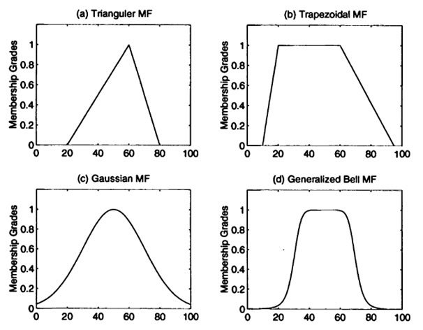
Figure 3. Examples of membership functions
So how do we read the membership function presented in Figure 2? For this reason, I invite you to look at figure 4 in which I choose some random examples of soil potential values. If the soil potential of my plot has a score of 0.5, it means that I consider it to be 60% in the “Low” class of the Soil Potential variable. If the potential is 3.5, 80% of it belongs to the “Low” class. What if the potential is at 7? Well, it belongs to 0% of the “Low” class.
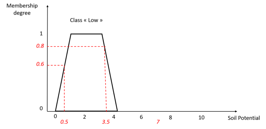
Figure 4. Reading and understanding of the membership function
How then to understand a soil potential with a value of 7? It is quite simple that here, we have only defined the membership function of the “Low” class, we have not characterized the entire soil potential variable! This is what we will do next, but just before that, let me define some terms related to the membership function (Figure 5).
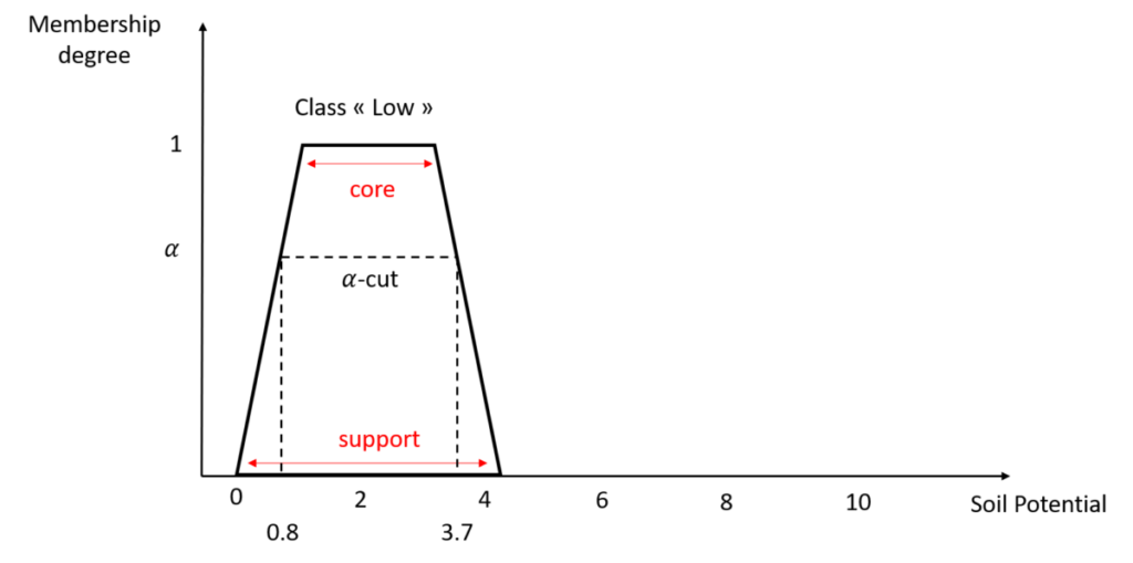
Figure 5. Terminologies of the membership function
A membership function is defined by two main parameters. First of all, its support: it is the set of values for which you will consider that they belong at least in part to the class studied. Here, values between 0 and 4.2 belong to the “Low” class with a membership degree greater than 0. The second parameter is the core, also called kernel: this is the range of values for which you consider that the values belong entirely to the class you are studying, and to no other class. In Figure 5, if the soil potential is between 1 and 3.5, then this soil potential belongs to the “Low” class with a membership degree of 100% [And in the case of a triangular membership function, this interval is actually only one value, the tip of the triangle – Figure 3]. Uh, hold on a minute!!! Basically, you’re telling me that a soil potential of 1.5 belongs entirely (100%) to the “Low” class but a soil potential of 0.5 belongs only in part (60%) to the “Low” class? Isn’t this all a little weird? It’s true that from this point of view, it raises questions. In fact, since we have defined the “Low” class of soil potential, this is how it is interpreted. There are two ways of looking at it. Either that suggests that a “Very Low” class could have been defined for soil potential, with values of soil potential lower than 0. Either, if we consider that a soil potential is necessarily greater than 0, well, we can redefine the membership function associated with the “Low” class of soil potential as shown in Figure 6. Does that suit you better?

Figure 6. Redefinition of the membership function to the “Low” class of soil potential.
And the last term presented in Figure 5: an alpha-cut is the range of values for which the values have a membership degree to the studied class greater than alpha. For example, in Figure 5, a 0.6-cut is the range of values from 0.5 to 3.7.
That’s it, we just have to expand the work we’ve just done for all the soil potential classes we want to define. For example, I defined 3 classes of soil potential, and therefore drew 3 membership functions to the soil potential variable (Figure 7). The set defined within the interval [0-10] composed of these three membership functions, for the soil potential variable is called the soil potential linguistic variable.
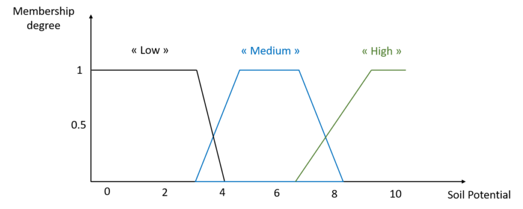
Figure 7. Linguistic variable Soil potential.
It is clear from this figure that some values have membership degrees defined for several classes. For example, a potential of 7 has a membership degree of 0 to the “Low” class, 0.7 to the “Medium” class and 0.2 to the “High” class. The sum of the membership degrees related to one specific value does not need to be equal to 1, it is not mandatory. And it is also not mandatory to have intersecting membership functions, one can totally imagine well separated membership functions over the range of possible values. Again, it all depends on how much expertise you have on your variables and how you interpret them.
Remember, we want to set up a fuzzy inference system to infer yield based on two input variables, soil potential and annual rainfall. So I still need to define my linguistic variables “Rainfall” and “Yield” (we also need to define a linguistic variable for our output variable, yield, and we will see why later!). This is done in the figure below. What you see here are my choices, which I propose to you as an example to support my point.
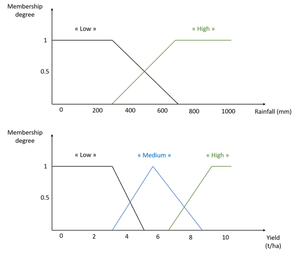
Figure 8. Linguistic variables Rainfall and Yield
Decision-making unit
We have already defined membership functions for the variables we are interested in, that’s not bad! Now, as we saw in the introduction, we need to define rules! These rules will explain how yield will behave according to our soil potential and rainfall variables. At the risk of repeating myself again, in our example, these rules are expertly defined! We will see that we can also infer rules, but that is not our objective here. We can therefore imagine that we have set up experiments and that we want to build a fuzzy inference system to formalize our experiments and results. This system will then be used to make new predictions, for example, when new data are available. Let’s imagine that I define the following rules:
- Rule 1: If the soil potential is high OR the rainfall is high then the yield is high
- Rule 2: If the soil potential is medium, then the yield is medium
- Rule 3: If the soil potential is low AND the rainfall is low, then the yield is low
An incomplete rule is a rule that does not use all input variables. This is the case, for example, with Rule 2. And that’s all right! As experts, we do not necessarily reason with all our input variables every time. And it is also not mandatory to have a rule for each use-case! It may be fine if we want a complete model but if we don’t want a model that is too specific to our data either, we have to be relatively flexible and not incorporate too many rules.
In these rules, we observe that we have the classic “If…, then…” but regarding rules 1 and 3, there are also two functions: “OR”, “AND”. So how to interpret these functions in our fuzzy inference system. If I have input values for soil potential and rainfall, how can I work with these rules? In the introduction, we had begun to try to feel what these functions “OR” and “AND” meant and had in particular brought them closer to the notions of “union” and “intersections” of intervals respectively. For rule 1 to be activated or fulfilled, it is necessary to have either a high soil potential or a high rainfall. But you don’t need both, only one of the two conditions is enough to activate the rule (it’s the “OR”). For rule 3 to be activated or fulfilled, both a low soil potential and a low rainfall must be present. We therefore need both conditions for the rule to be fulfilled (it is the “AND”). Once we have understood the difference between these two functions, let us now present two types of operators to take them into account:
- The operators of Zadeh (Lotfi Zadeh proposed them):
- Synthesize the notion of union (it is the “OR” function) by the maximum of the membership degrees to the classes considered
- Synthesize the notion of intersection (it is the “AND” function) by the minimum of the membership degrees to the classes considered
Let’s show with an example example what happens with rule 1. Rule 1 is activated if and only if the soil potential is high OR the rainfall is high. Imagine that I have a “high” soil potential, say 8, and a “high” rainfall, say 600mm (Figure 9).
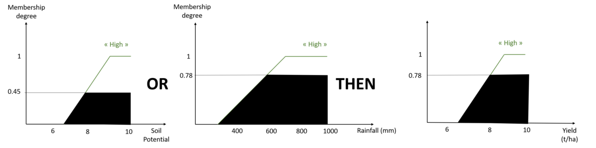
Figure 9. Activation of rule n°1 of our fuzzy inference system
If rule 1 is activated, then the yield is high, as shown in the figure. And the corresponding membership degree is the maximum of the membership degrees of our input values in the “High” soil potential and rainfall classes. If, in Rule 1, we had had the “AND” function instead of the “OR” function, the final degree of membership in the “High” yield class would have been 0.45 and not 0.78, since the minimum of the degrees of membership would have been applied. In this example, we look at membership in the “High” yield class simply because that is what Rule 1 tells us! If I had defined the rule “If the soil potential is high OR the rainfall is high, then the yield is medium”, I would have obtained the following figure:
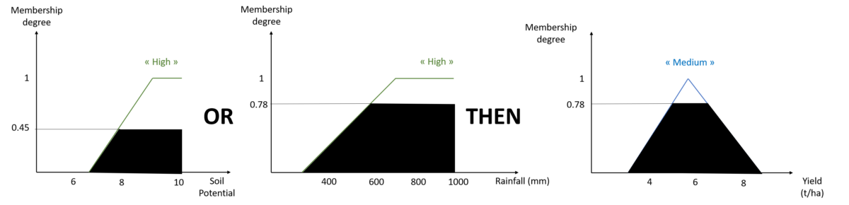
Figure 10. Another example of rule activation
And I wouldn’t have been interested in the “low” and “medium” soil potential classes, or the “low” rainfall class even if they overlapped, simply because Rule 1 doesn’t mention them!
- The second types of operators are the so-called probabilistic operators, they:
- Synthesize the notion of union (it is the “OR” function) by the sum of the membership degrees to the classes considered less the product of the membership degrees to the classes considered
- Synthesize the notion of intersection (it is the “AND” function) by multiplying the membership degrees to the classes considered
If we use the example given in figure 9:
- Using Zadeh operators, activating rule 1 with our example, the membership degree to the “High” yield class was 0.78. It was the maximum of the membership degrees: max (0.45 ; 0.78)
- Using the probabilistic operator in the same way, we would have obtained the membership degree 0.45+0.78 – 0.45×0.78 = 0.879
The choice of operator therefore has an influence on the membership degree obtained for the output! Each user will choose the type of operator that will best match his or her expertise. We realize that the Zadeh operator is a little more brutal in the sense that only one of the input membership degrees is used to calculate the output membership degree. With probabilistic operators, there is a little more of a compromise idea since all input membership degrees are used.
In our example of yield inference, we have defined 3 rules (rules n°1 to 3). For a new pair of input data (Soil Potential; Rainfall), it will be possible to infer a yield according to the activation or not of the rules that have been set. As shown in Figures 9 and 10, when a rule is activated, a fuzzy set is obtained as output (this is the kind of black mass drawn on the figures). What can I do when several rules are activated at the same time? In other words, how can the result of these rules be combined? And above all, in view of our initial problem, how to characterize the output yield of our inference model, i.e. what will be the expected output value? We’ll see all this in the last brick of fuzzy inference systems: defuzzification.
Defuzzification
To fully understand what we are facing, let us consider that we have put in place our fuzzy inference system. We therefore have a set of linguistic variables (those we defined above) and a set of associated rules (these are rules 1, 2 and 3 in the previous section). A yield can now be inferred from a combination of soil potential and rainfall values. Let’s see what’s going on. Imagine that during a new field experiment, we measured a soil potential of 7 and a rainfall of 500mm on a plot.
According to our linguistic variable Soil Potential, we realize that a value of 7 corresponds to a membership degree of 0 to the “weak” class, 0.7 to the “medium” class and 0.2 to the “high” class. Similarly, according to our linguistic variable Pluviometry, we realize that a value of 500mm corresponds to a membership degree of 0.5 to the “low” class, and 0.5 to the “high” class. By following the fuzzy inference rules that have been defined, we observe that:
- rule 1 is activated because the condition “high” soil potential OR “high” rainfall is respected
- rule 2 is activated because the condition soil potential “medium” is respected (the corresponding membership degree is greater than 0, it is 0.7)
- rule 3 is not activated because the membership degree to the “low” class of the Soil Potential set is 0 and the membership degree to the “low” class of the Rainfall set is 0.5. Both conditions must be met for the rule to be activated in view of the “AND” function of the rule.
Graphically, we have the following figure for these three rules:
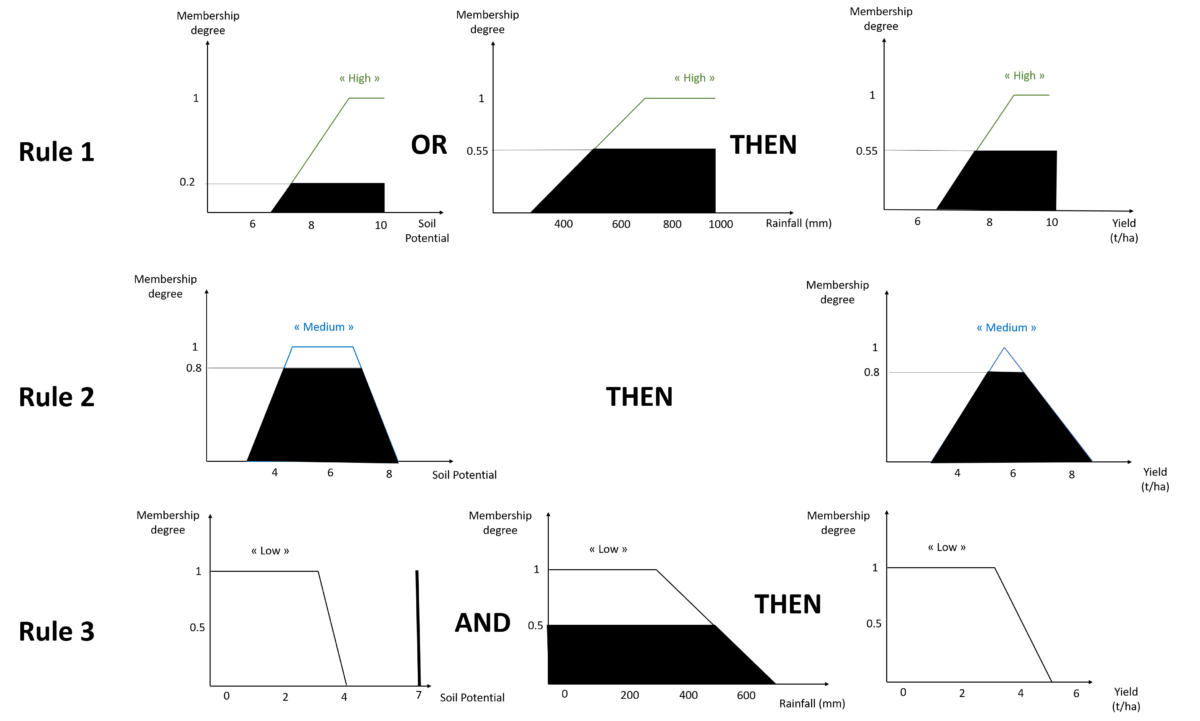
Figure 11. Yield inference from new input data regarding the inference rules previously defined
By combining the three outputs, we arrive at the following complete inference:
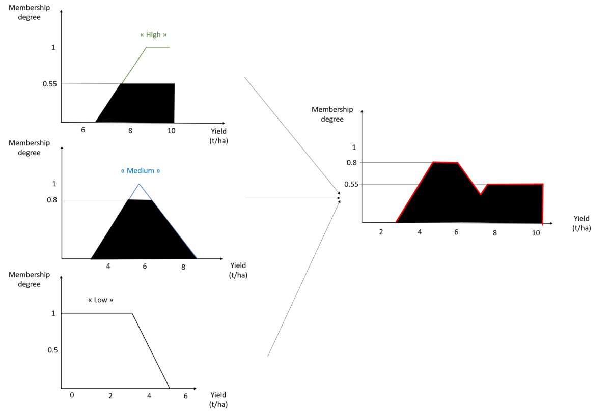
Figure 12. Combination of yield outputs for the pair Soil Potential; Rainfall (7; 500). Be careful with the abscissa values.
As discussed above, the defuzzification step will consist in transforming the fuzzy set of yield into a final crisp yield value for our pair Soil Potential; Rainfall (7; 500). Several defuzzification methods exist, but I will only present two of them, which are the mainly known ones.
The first one is the average method of maxima (MM). In this method, the output is calculated as the average of the abscissa values for which the membership degree is maximum. In the example in Figure 12, we therefore look at the maximum membership degree (0.8) and the corresponding abscissa yield values (the interval [5-6.5]). The final yield is obtained by calculating the average of the interval, i.e. (5+6.5)/2=5.75 t/ha
The second method is the Center of Gravity (COG) method. In this method, the output is calculated as the abscissa value of the centre of gravity of the surface under the curve (the red curve), here around 6.2 t/ha.
As with operators, we realize that the defuzzification method impacts the crisp final output of the fuzzy inference system. It is up to the user to choose the most appropriate method according to him. The average method of maxima is quite brutal, only the maximum membership degree is considered. The centre of gravity method is more flexible since the entire fuzzy output is taken into account when calculating the defuzzification output. We can see this method as a kind of interpolation. However, it is more time-consuming to calculate, which is normal since it has to calculate a centre of gravity.
As a discussion and conclusion
After having built a fuzzy inference system (setting up the membership functions, establishing fuzzy inference rules, defuzzifying the fuzzy outputs of the system), we are therefore able to infer a yield output value from new soil potential and rainfall input values. If we try to take a step back, what are the big advantages of fuzzy inference systems?
- Expertise can be incorporated into your model through membership functions and inference rules!
- Non-linear phenomena can be modelled! None of our membership functions or rules had linear behaviour. We can therefore model complex phenomena.
- We can play on the fuzziness and uncertainty of our data with the membership functions. Imagine, for example, that you know the measurement uncertainty of your sensor. For example, you can model the data you collect with a membership function. As a consequence, you do not have a single value at the output of the sensor but a set of values with a membership degree given by your membership function. It is also possible to imagine working in two dimensions with the uncertainty associated with the positioning of an agricultural machine in the field (Figure 13). We then define in the same way a core and a support for the membership function but in two dimensions.
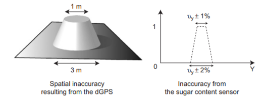
Figure 13. Consideration of the uncertainty associated with the positioning of an agricultural machine (left) and the uncertainty associated with measuring the berry sugar content with a sensor (right). From Paoli et al, (2007). Spatial Data Fusion for Qualitative Estimation of Fuzzy Request Zones: Application on Precision Viticulture. Fuzzy Sets and Systems, 158, 535-554.
In all this blog post, I assumed that we had the expertise to generate the fuzzy inference rules. In other words, I considered that we had worked in a so-called “supervised” way. We have input data, we build membership functions, we know the rules of our fuzzy inference system and we use that system to produce estimates. Nevertheless, it is possible to work with fuzzy logic in an “unsupervised” way. In this case, based on the membership functions that we define (we have to define some membership functions however, unsupervised learning models cannot invent them because it is our expertise), the model can find the most appropriate rules for our fuzzy inference system. The problem we can have by working in this way is that our model can generate a lot of rules, which can make the understanding of the system relatively complex… Nevertheless, some algorithms exist to try to optimize or simplify the generated rules in order to clarify the fuzzy inference system. One can understand that if we generate a lot of rules and no one is able to interpret them, it doesn’t really matter… Once again, the objective is not to end up with too many rules, otherwise the model will not be usable or generalizable to other data than those that were used to built it (it’s always the same overfitting problem).
To work on fuzzy logic aspects, several options are available to you, but I advise you to start with the FisPRO software (https://www7.inra.fr/mia/M/fispro/fispro2013_en.html) developed by an INRA team and which offers an interface that is fairly easy to use to set up fuzzy inference systems.
![]()
One final point of attention: I hope I have been quite clear that the input variables used in a fuzzy inference system must be quantifiable or significant on a scale (numerical values are required). The point I raise here refers to the use of absolute or relative variables. When working with agro-environmental data, if you come to use a variable such as elevation or conductivity, you will always have to refer to a particular context. For example, saying that an elevation is low or high does not really make sense. A high elevation in one place may be considered low in another. It is therefore sometimes more interesting to work in a relative rather than in a absolute way. For example, if you work with within-field datasets, it might be better to use deviations from the average elevation of the plot rather than with the raw elevation values as they are.
Support Aspexit’s blog posts on TIPEEE
A small donation to continue to offer quality content and to always share and popularize knowledge =) ?