As you are no doubt aware, geo-positioning has been a particularly powerful lever for many agricultural applications and crop itineraries. But are you clear on the extent of geo-positioning systems, tools and methods? If you’re French, you should be crazy about abbreviations – so hang on : GPS, GNSS, EGNOS, DOP, TTF, SBAS, LBAS, WAAS, RTCM, CMR, dGPS, RTK, MAC, VRS, PPP, PPK, nRTK, RTX, PPP-RTK, NTRIP… Want more? After a lot of cross-checking of sources from scientific articles, forums, blogs, reports, or seminars, I bring here my contribution to try to lift the veil on the subject. This article may seem a bit like a catalogue, but I will try as much as possible to make the link between the parts so that the reading is pleasant! Of course, I’ll take the opportunity to discuss a little about Precision Agriculture.
The constellations of navigation satellites
Without satellites, it would be relatively difficult to position oneself precisely on the surface of the globe. And satellites, there’s starting to be a lot of them… The constellation that everyone has in mind is certainly the constellation straight from the United States – GPS [Global Positioning System] – originally known as Navstar GPS [Navigation Satellite Time and Ranging], so the Americans have slightly simplified the name. It should be kept in mind that the GPS constellation is American; in fact, we have to talk about GNSS [Global Navigation Satellite System] to be broader and extend the name to all the world’s satellite constellations. The GPS constellation has been operational and usable for public activities since the mid-1990s. At that time, it consisted of 24 satellites in orbit, each classified in a block (Block I, Block II, Block IIA, Block IIR, etc.) representing the generation of satellites of which it was a part. At the time of writing, 32 satellites make up the GPS constellation – these satellites being distributed in three independent orbits. For quite obvious strategic and geopolitical reasons, the world’s major powers have also launched their own constellation so as not to be dependent on the positioning systems deployed by the Americans (Figure 1). The Russians have set up their “GLONASS” constellation (24 satellites), the Europeans “GALILEO” (26 satellites), the Chinese “BEIDOU” (35 satellites), the Indians “IRNSS” (7 satellites) and the Japanese “QZSS” (3 satellites). When you start summoning all these satellites, it starts to make a hell of a bunch. These constellations are not yet all fully operational – they are working, of course, but a few more satellites will be added (the GALILEO constellation, for example, is still waiting for 4 more). And these constellations are not independent, quite the contrary. Some so-called multi-constellation solutions take advantage of satellites in different constellations to improve the quality of the signal received. The reason is quite simple: if the satellite signal receiver at Earth level picks up more satellites, the positioning accuracy can only be improved – we’ll come back to this later!
Generally speaking, navigation satellites are positioned in two main orbits: the geostationary orbit (GEO) and the medium earth orbit (MEO), the vast majority of which are nevertheless positioned in a medium orbit:
- The geostationary orbit around the Earth is located at an altitude of nearly 36,000 km. A satellite in a geostationary orbit, known as a “geostationary satellite”, then moves at the same speed as the Earth’s rotation and therefore appears fixed above a certain area (this specific area is called the satellite’s coverage area). Geostationary satellites are therefore ideal for covering a fixed area on the Earth (a parallel can be drawn with so-called Earth observation satellites, which are rather on a sun-synchronous orbit, which means that they always pass over a given location at the same local solar time).
- The average orbit around the Earth is at an altitude of around 20,000 km. At this altitude, the satellite takes between 2 and 12 hours to circumnavigate the Earth. The advantage of this orbit is that it is very stable, and the signals sent by the satellite can be received over a large part of the surface of the Earth.
Why choose a medium orbit rather than a low or geostationary orbit? Compared to the geostationary orbit, a fairly simple first answer is that it requires a much less powerful satellite launcher (there are a few thousand kilometres less to travel, which is not completely negligible…). A second answer has more to do with the time it takes for the signal emitted by the satellite to reach Earth – this is called “latency”. From a geostationary satellite, the signal makes a round trip in 240 milliseconds. This latency is reduced to nearly 50 milliseconds from a medium orbit. And depending on the applications imagined, reducing this latency can be very interesting! In low orbit, this latency could be even lower, but given the closer coverage of satellites in low orbit (they see less since they are lower in altitude), many more satellites would be needed in low orbit than in medium orbit. Let’s say then that the medium orbit for navigation satellites is a rather good compromise.
What do the satellites transmit to us?
Each satellite transmits two types of messages: the almanac and the ephemerides. The almanac consists of general information on the location and health of the satellite in the constellation. A GNSS receiver with an up-to-date almanac therefore knows approximately its first position, the day and time, and therefore knows where it has to scan space to search for the satellites. Ephemerides, on the other hand, consist of precise information about the satellite’s position used to make the distance calculation measurements. Each satellite transmits its own ephemerides. Both the almanac and the ephemerides are essential for the GNSS receiver to locate the satellites, acquire the signals, and calculate your geographic position.
The satellites of the different satellites transmit signals continuously on different frequencies corresponding to specific wavelengths. In the case of GPS, this is for example on the frequencies L1 (1575.42 MHz) and L2 (1227.60 MHz) – for Galileo we speak of the frequencies E1, E5 or E6. Satellite signals contain two main types of information: (1) the PRN (Pseudo Random Noise) codes, which identify the satellite and calculate the distance between the satellite and the receiver, and (2) navigation messages, which provide precise information on the location of the satellite (Figure 1). The PRN code used for civilian applications is known as the “C/A code”, while the one used by the military – and encrypted – is known as the “P code” (the C/A code is transmitted only on frequency L1, while the P code is transmitted on frequencies L1 and L2). The PRN codes are a sequence of 0 and 1, specific to each satellite, and can be understood as a signature, very precisely located in time, of each satellite. The codes have a random appearance – hence the name Pseudo Random Noise – but in reality do transmit precise information. A receiver is therefore able, based on a portion of the PRN code, to recognize the signal, to know which satellite it was transmitted from, and to know its very precise transmission schedule. By comparing this satellite transmission schedule with the reception schedule at the receiver, it is possible to deduce the duration of the travel and therefore the distance between the receiver and the satellite, since the propagation speed of the radio signal is known (speed = distance / time). To be precise, we speak rather of pseudo-distance between the receiver and the satellite, rather than distance, because the travel time is not perfectly accurate (there may be discrepancies between the atomic clocks of the satellites, and the less accurate clocks at ground level).
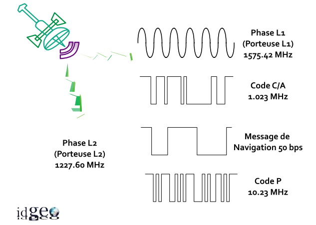
Figure 1: Signal structure of a GPS satellite. Source: IDGEO (Institut de Développement de la Géomatique), presented in Lahaye and Ladet (2014).
We have just seen that by using the C/A code and the pseudo-distance between GNSS receiver and satellite, we were able to position ourselves. And that’s pretty cool! Nevertheless, with this type of positioning we are often limited to accuracies of the order of a meter (metric precision). When you want to be more accurate, especially when the GNSS receiver is in motion, you have to change the method, and use the phase of the signal (reminds you of some old high school physics courses?) rather than its code (Figure 2). For your information, this is what we do with the RTK! In this case, we work with the whole sine wave characteristic rather than the simple code that is transported, so basically, there is a way to be more accurate! More than the phase, it is mainly the phase shift between the signal emitted by the satellite and the signal received by the receiver that interests us. The offset, in itself, doesn’t seem that complicated. It is enough to shift the received wave in time for it to match the transmitted wave. The phase shift, okay, but how many oscillations exactly? On a sinusoidal wave, when I have put the two waves in phase, I can shift one oscillation and I’m still in phase; the same with two, three, four, etc. oscillations. Here, it becomes much more complex, and that’s what we call ambiguity. All the methods that work with the phase of the satellite signal to improve positioning seek to lift the veil of ambiguity. The question we’re looking for an answer to is: How many oscillations were there between the transmission and reception of the signal? If you’re interested, you can look at the methods of wave fronts emitted by the satellites, fronts that are crossed to estimate the operator’s position as well as possible, knowing that the operator’s position does not change while the satellites are mobile in space. But we will not go further than that in this article!
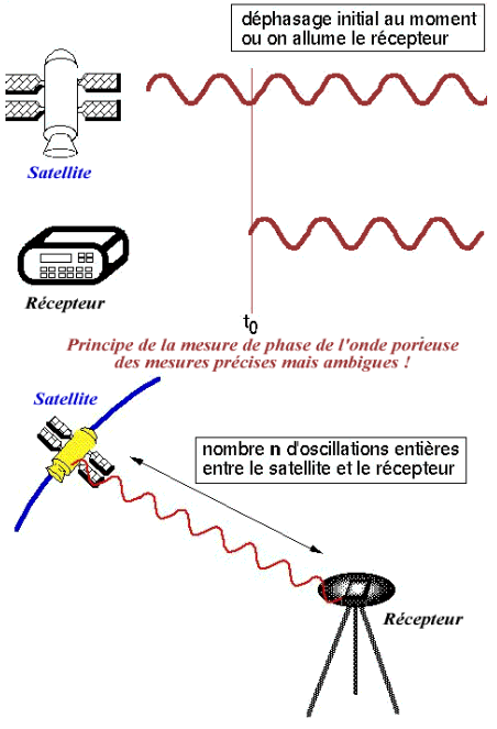
Figure 2. The ambiguity of the GPS signal. Source: Planet Earth – ENS de Lyon
Sources of positioning error
The satellite therefore transmits its signal to a receiver on Earth, which analyses the signal and derives a position from it. Too simple, isn’t it? If we want to position ourselves with an accuracy of +/- 100 metres, we can say yes. Wow! There are actually a large number of potential sources of uncertainty and error that limit the accuracy of positioning.
The calculation of geopositioning can be based on two measurements: (1) either the measurement of the time it took for the signals emitted by at least four satellites to travel the distance separating them from the mobile, (2) or the phase shift of the signals, in which case very sophisticated equipment has to remove ambiguities (number of oscillations between the emission of the signal by the satellite and its reception by the mobile). Theoretically, (1) must give decimetre accuracy and (2) must give millimetre accuracy, but sources of error interfere with this accuracy.
Here are the main ones:
- Atmospheric sources of error: Before reaching the ground, satellite signals must pass through the atmosphere (Figure 3), including two of these layers; the troposphere and the ionosphere. In the troposphere, humidity and pressure variations change the tropospheric refractive index, and therefore impact the speed and direction of signal propagation. The ionosphere is not really a layer in itself but rather characterizes various layers of ionized particles and electrons found at altitudes of 80 to 250 km in the atmosphere. These layers ionized by solar radiation (especially X-rays and ultraviolet radiation) also change the speed of signal propagation. Note that ionospheric disturbances are the most troublesome, and that areas close to the equator are the most affected by these problems.
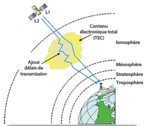
Figure 3: Effects of ionospheric refraction. GPS signals are affected in different ways, depending on whether they are codes or phases. Source: Reflections. University of Liège.
- Errors in satellite geometry: When the satellites are well distributed in the sky and no obstacle disturbs their visibility (mountains, buildings…), the geometry of the satellites is considered to be rather good. In a perfect world, if we knew the distance from a receiver on Earth to several visible satellites, we could find the precise positioning of this receiver by crossing the circles around each satellite (the circles would have as radius the distance from the satellite to the receiver). We would then have a single point when the circles intersect. Unfortunately, with the geometry error of the satellites, we have more of a small area than a point. The effect of satellite geometry on positioning errors is called DOP (Dilution of Precision). DOP is sometimes present in Precision Agriculture datasets, so be sure to take a look at them. There are not really any reference values for DOP values although quite generally, it is considered that 1 to 2 is excellent, 3 to 4 is good, 5 to 7 is acceptable and 8 or more is poor. It really depends on the field application, it’s still a trade-off… You can even sometimes find information about satellite geometry errors that go a bit further than the DOP. For example, you can find HDOP, VDOP, PDOP, TDOP or GDOP values, which respectively clarify the horizontal, vertical, position, time and geometric error.
- The so-called multipath errors: This source of error can be understood quite intuitively. It is the fact that the signal arriving at the receiver on Earth can follow several different paths, especially if it “bounces” off obstacles. Because of these multiple paths, it is difficult to trace the true distance of the satellite from the receiver. And there are many such obstacles: atmospheric channelling, ionospheric reflection and refraction, and the reflection of a body of water, mountains, or buildings. And in the agricultural world, we can add forests, wind turbines …
- Timing and satellite orbit errors: All satellites have very precise atomic clocks and follow certain orbits (geostationary and medium orbit; this was discussed above). The problem is that small clock and orbit drifts are unavoidable, and must be considered to correct the signals received at Earth level.
Differential corrections
Fortunately, a number of people have characterized these sources of error and proposed corrections! We’re going to be able to be a little more precise than +/- 100 metres, are you reassured? We will be able to distinguish two main families of differential corrections:
- The LBAS (local-based augmentation system). We can also see GBAS being passed as “ground-based augmentation system” but it is the same thing.
- The SBAS (“satellite-based augmentation systems” or “spatial augmentation system” in French).
Before going into detail (don’t worry, you’ll get your money’s worth!), understand roughly, as the name suggests, that the LBAS is based on a local reference station whose antenna is installed at a known location, and that the LBAS corrections are then sent to a mobile receiver (e.g. on a tractor) in real time or as post-processing via radio networks or the internet. In the LBAS corrections, we will therefore find dGPS, RTK and all its derivatives; we will come back to this later! In SBAS, satellite signals are received at receivers and transmitted to processing centers for correction. These corrections are sent to the geostationary satellites via control stations, and it is the geostationary satellites that rebroadcast the corrections to the mobile receiver (smartphone, tractor…). So there is no need for reference stations near where you want to position yourself. It is in the SBAS that we will be able to find the EGNOS corrections (and foreign inclinations), and the corrections quite known in agriculture Omnistar, and SF1/SF2… The SBAS is also a differential correction! Come on, let’s get into the thick of it!
SBAS – Satellite-based augmentation systems
EGNOS and global cousins
With SBAS, it is therefore the geostationary satellite that sends back the positioning corrections (which it has itself received) to GNSS receivers in the field. SBAS signals are of the same nature as GNSS signals – this is why the GNSS antenna receives both GNSS and SBAS signals in parallel – and are therefore also sensitive to the same types of obstructions. Transmitting data on the same frequency as GNSS signals has a big advantage: only one antenna is needed on the receiver! Let’s take a look at the SBAS differential correction services, with a special focus on EGNOS, and then on some rather agriculture-oriented services:
EGNOS (European Geostationary Navigation Overlay Service): This is the European SBAS system (visible from all over Europe, but depending on the topography of the terrain, satellites are sometimes not clearly visible so EGNOS correction does not happen). EGNOS is free and the corrections are broadcast on the L1 carrier of the GPS signal (see paragraph “What are the satellites transmitting to us?”), so there is no additional antenna required on the receiver to receive EGNOS. This is the GPS constellation and not the GNSS constellations of the whole world, because for the moment EGNOS is not interoperable with Glonass or Galileo – but this will be the case in the long term, so the EGNOS correction will also increase the positioning via Glonass and Galileo [it will be the E1 carrier of the Galileo signal]. EGNOS is interoperable with SBAS systems in other parts of the world. Note for information the other SBAS constellations in the world: “WASS” (USA), “MSAS” (Japan), “GAGAN” (India), “SNAS” (China).
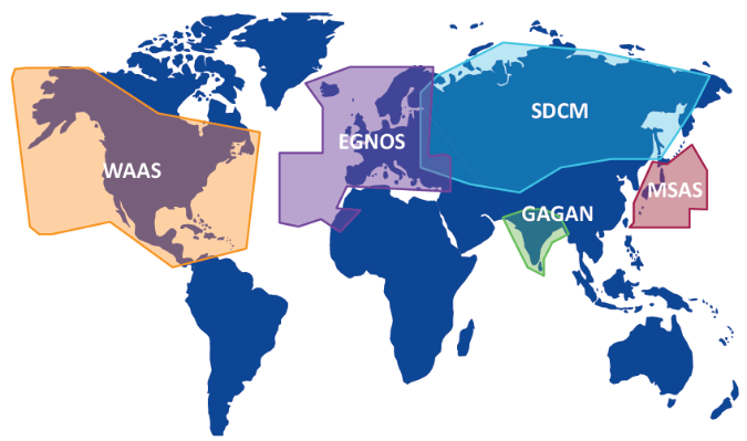
Figure 4. Global SBAS.
The performance of EGNOS is measured every day. Under good conditions, EGNOS is considered as a correction allowing sub-metric positioning (accuracy to within 1 metre) with a 95% confidence interval (in 95% of situations this is the case). This accuracy can even go down to 20-30 cm in a situation called “pass to pass” rather specific to agriculture, where one is interested in the accuracy observed within a 15-minute time window – i.e. between a first and a second machine pass (pass to pass) at the same place in a short time interval.
The 2 major advantages of EGNOS that have already been discussed a little: (1) it is a free correction, (2) no dependence on radio and GPRS channels to transmit corrections since everything is transmitted by geostationary satellites. Note that a paid service based on EGNOS also exists. This is the EDAS NTRIP service, which provides free DGNSS and RTK corrections in the vicinity of EGNOS reference stations. Be aware, however, that in this case, the NTRIP communication protocol is used – DGNSS and RTK receivers must therefore be compatible with this protocol .
Small precaution of use: Every six to twelve months, the intermediary through which the EGNOS correction passes changes (the frequency of diffusion is no longer exactly the same). You should therefore remember to check the receiver’s settings and change them accordingly because the change is not automatic.
For your information, the arrival of powerful GNSS chips dedicated to smartphones may help democratize the use of EGNOS. You can see if you are picking up this correction using the GPS-Test application. If your smartphone is compatible, you will be able to see a “SBAS” line at the bottom of the application. You may not be able to receive an SBAS satellite in your area, even if your phone is compatible. To find out, you have to check if two components of your phone are compatible: the GNSS antenna, and the SoC. One retrieves data, the other processes and formats it. If one of the two is not compatible, you cannot have SBAS correction on your phone.
Agriculture-oriented SBAS
With regard to geopositioning in agriculture, it is interesting to note that nearly 80% of the sector’s guidance systems integrate the EGNOS correction – so it is available! In addition to EGNOS, several structures have proposed geolocation services dedicated to agriculture :
- In particular, Fugro provides OmniSTAR VBS corrections (single-frequency antenna; 15-30 cm accuracy), and OmniSTAR XP and Omnistar HP (dual-frequency antenna; 10-15 cm accuracy). OmniSTAR signals are compatible with the vast majority of GPS receivers.
- John Deere provides the SF1 (free) and SF2 (subscription) correction signals. These signals should soon no longer be available for some John Deere StarFire antennas (StarFire is quite similar to the American WAAS SBAS). A new signal – SF3 – will be made available on the new antennas.
LBAS – Local-based augmentation systems
I put a layer of it here but within the LBAS, and contrary to the SBAS, the corrections are calculated from a local reference station, and applied to the mobile receiver, either in real time or in a post-processing software, via internet or radio. Therefore, a station close to home is required to be correctly located (Figure 5). In the same way with SBAS, we work well with satellite signals! In the LBAS, there are a lot of people: we will go back to the RTK for a while and have a look next to it with the nRTK and the PPP.
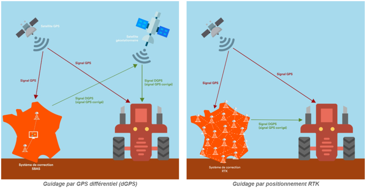
Figure 5. Difference between an EGNOS-type SBAS system and an RTK positioning system. Source: Teria
RTK
With RTK, the aim is clearly to achieve very precise geolocation (in this case, we use the phase and code of the satellite signal rather than its code only – see the paragraph: “What are the satellites transmitting to us? ” ; with EGNOS, for example, we are only interested in the signal code). There are several ways of looking at RTK. You can have two types of RTK base stations: either placed by the user, or managed by a private third party (this is called nRTK for Network RTK – we will come back to this in the next section). In the case of a user-placed station, the station is placed on a known point and sends corrections to the receiver by radio. The station is then usually very close to the receiver and the error is as small as possible. Nevertheless, it is necessary to know very precisely the point on which the station is placed. If the station is placed in a corner of the plot – this is known as a mobile base – it is important to make sure that it can be placed in exactly the same place to avoid problems of repeatability in the event of re-cultivation. If the station is fixed on a building – this is called a local base – the previous problem is no longer a problem, but it is nevertheless necessary to ensure the stability of the antenna, good observation conditions, and a good range of radio waves to transmit the corrections (even if it means installing repeaters in the geographical area to broadcast the corrections to the final receiver if there are obstacles to avoid). RTK stations can also be distinguished according to the way in which the corrections are sent to the receiver :
- « radio » RTKs where corrections are sent by radio, and which may require a fee from the French regulatory authority for electronic communications and postal services (ARCEP). The transmission of radio signals from RTK bases can be carried out on two free frequencies, intended for surveyors, provided that it is discontinuous in time (temporary use of these so-called “roaming” frequencies). As these frequencies are public, any compatible GPS receiver can pick up the signal from the RTK base as long as the correction is not encrypted. If the two frequencies are already used by neighbouring RTK bases, the third base will necessarily use a common frequency. An RTK guidance system within the range of the two bases using the common frequency will be completely lost. It will no longer know which signal to use. To avoid this problem, it is necessary to request the allocation of a frequency from ARCEP against an annual fee. With the multiplication of bases, the availability of frequency becomes problematic.
- The RTK “GPRS”, RTK “GSM”, RTK “Telephone”. In this case, the correction is transmitted to the tractor via the mobile phone network (GPRS). The tractor is then equipped with a GSM antenna and a modem which receives a single or multi operator SIM card. The multi-operator solution makes it possible to avoid areas not covered by certain operators.
- RTK GPRS “multibase” or GPRS “network”: We are in the case of nRTK here, we will discuss it again in the following section.
Using RTK correction systems requires an interest in notions of hardware compatibility. Above all, the receiver must be able to receive and process corrections by being an RTK client (which is not currently the case for most smartphones). In the case of agriculture, it is necessary to ask whether the console is capable of managing the correction, whether the antenna is capable of picking up the correction, or whether the tractor brand is compatible with any correction. It should also be kept in mind that receivers installed on agricultural machinery already have the capability to receive RTK corrections. However, centimeter and RTK corrections often require a console unlock to be active – the cost of this computer key to unlock the functionality can sometimes be high.
The transmission format of the RTK signal must be comprehensible to all receivers of the network users. The problem (quite common in agriculture, by the way) is that most manufacturers use a proprietary format, which cannot be used (or fully used) by competing systems. Under conditions where the base and the receiver belong to the same manufacturer, the correction is transmitted in the manufacturer’s format, unknown to the user in most cases. As a result, many farmers cannot benefit from the RTK service due to incompatible equipment. However, the US Army has been developing a universal format for quite some time now: the RTCM (Radio Technical Commission for Maritime Services). Among the proprietary formats, the Trimble format (CMR, CMR+ and CMRx) has become a standard format, but it remains the partially open proprietary Trimble format, which can be modified at any time by its designers.
Some additional definitions to keep in mind :
- Hold signals are corrections that take over for a short period of time (1-20 minutes) when the RTK correction is cut. These signals can be algorithms in themselves, or another type of correction.
- The time to first fix (TTFF or TTF) is the waiting time necessary for the correction to be operational after the console is switched on. Not all corrections are concerned. This waiting time can be up to 25 minutes.
nRTK: RTK networks
With the RTK, we saw it, we need a local reference station! And if we don’t have the financial, logistical or material means to have one of our own, well, it’s starting to get a bit complicated. We can add a lot of disadvantages to the fact of having RTK beacons: you need to have 2 GNSS receivers and a clear and known point in coordinates; you need to have the base monitored, the base has a limited range; you need a relevant telecommunication link such as radio (UHF) and you need a user license from ARCEP. This is why several structures have developed a network of stations on French territory. Instead of speaking of RTK, we then speak of nRTK (“n” for “network”). With this, geo-positioning is outsourced to these structures; no more need to bother with a station, the investment and operational implementation costs on the base are limited, there is no need for UHF radio licences and there is also less of a problem with the availability of correction using existing telecom networks and mobile operators. All that is required is to pay a geolocation subscription.
The principle of nRTK consists in retrieving data from the network RTK databases in real time on a central computer server via a telecom network. When the tractor’s guidance system is switched on, it sends its position to the central server via mobile telephony. This initial location allows the user’s working area to be located. The server then calculates a correction for the field being worked using the permanent data from the stations in the network and adapts this correction according to the movement of the tractor within the network. Several correction concepts exist, each with its own calculation methods (“MAC” for Master Auxiliary Concept or Master Slave; “VRS” for Virtual Reference System or Virtual Station; and “FKP” for Flächen Korrektur Parameter or Area Correction Parameter). For information, the MAC concept is used by the Orphéon network, the FKP concept by the Teria network and the VRS concept by the Sat-info network (see the list of nRTK networks just after). The corrections are then transmitted by the GSM/GPRS type mobile phone network, which requires a modem in the tractor and the use of a compatible guidance system (corrections can also be transmitted by radio, but in this case it is often necessary to contact ARCEP – see the paragraph on RTK).
These are the main nRTK networks that can be found in France :
- Orpheon Network: This is the first full GNSS nRTK network in France, with more than 160 operational stations in mainland France (the reference station closest to the user is never more than 30 km away on French territory). The network of stations is owned by the company Geodata Diffusion. This company also deploys the “Precisio” service, an agricultural equipment self-guidance service, from the Orpheon station network. Precisio is available in several offers (MSPRé, FLEXPRé, OPTIPré) and is compatible with all brands of self-guidance and agricultural equipment, compatible with GPS, Glonass, Beidou and Galileo technologies. Access to the correction would also be instantaneous, i.e. without convergence time (the famous Time to First Fix). Orpheon announces an expected accuracy of 1 standard deviation between 1-2 cm in planimetry (Lambert 93) and 2-3 cm in altimetry (IGN69). The Orpheon network is based on the Master Auxiliary Concept (MAC), i.e. reference stations in the same area have a number of corrections in common – for example satellite or atmospheric corrections.
- Teria network: this is a network of surveyors, operating on a principle quite similar to that of the Orpheon network. Teria offers several solutions, including (1) “TERIAsat”, a 100% GNSS satellite service. The corrections can be received either via an external box or directly in certain receivers integrating a TERIAsat-compatible L-Band modem, and (2) “TERIAmove”, which is designed to meet the precision location requirements for all receivers with a moving GNSS antenna. There is therefore a strong interest here in the context of precision farming.
- Satinfo Network: the network of stations developed by CLAAS. The network includes more than 200 permanent GNSS stations in France to provide DGPS or RTK corrections up to centimetric resolution. SatInfo offers the RTK NET service.
- VRS-tec Network: Trimble’s station network provides a service similar to the CenterPoint service (but here with a station network as opposed to the simple RTK service).
- Centipede Network: this is an open source RTK network, so it is worth mentioning – even if there is relatively little information about it at the moment.
The term VRS used in the name of the Trimble network – for Virtual Reference Station – reflects the fact that reference stations of known location model a geolocation error at the user level by creating a virtual station where the user is located (and therefore acting as if there is a reference station near the user).
Depending on the station networks, and in the same way as for RTK, data exchanges can be carried out via the Internet (2G, GPRS, 3G) or radio. The networks often have partnerships with telephone operators, simply because they cover the whole territory relatively well. The French regulatory authority for electronic communications and postal services (ARCEP) announces in particular that 98.4% of the territory is covered in 2G by at least one operator.
Certain standards exist for disseminating positioning information. This is notably the case of the NTRIP protocol for data exchange and the RTCM format for the dissemination of corrections (we often speak of RTCM dissemination via NTRIP because the acronym NTRIP means Network and Transport of Rtcm via Internet Protocol). In order to receive corrections to NTRIP, the client receiver must also be NTRIP-compliant. Another interest of NTRIP is to be able to provide correction data to a very large number of customers. There is no need to invest in your own hardware. GNSS observations are often stored in Rinex format files.
PPK
The principle is the same for RTK but the correction data is not transmitted live. It is stored in a file in Rinex format on the base, which makes it possible to calculate the coordinates of a point parked by the user using post-processing software. Teria, Oprheon or IGN offer Rinex files linked to their bases. The advantage is that the data is free of charge for the IGN, or that no 3G-4G connection is required.
PPP
The main difference between PPP (Precise Point Positioning) and RTK is that PPP uses a single GNSS receiver whereas RTK uses a local reference station (fixed or mobile) in addition to a GNSS receiver. With PPP, geopositioning is therefore not dependent on the availability of data from reference stations in the vicinity of the user. Nevertheless, PPP and RTK differential corrections should not be seen as competitors. They are also intended to be combined, which will be discussed in the following section PPP-RTK.
Be careful, I left PPP in the LBAS section to understand the differences with RTK, but PPP is much closer to a SBAS than a LBAS since there are no local reference stations.
PPP will tend to use dual-frequency receivers (whereas RTK broadcasts on a single frequency – the L1 carrier in the case of GPS). To understand the benefits of multi-frequency, consider that the delay of a signal depends on its frequency, so if we send several signals at different frequencies, we can better model disturbances (everything that happens in the ionosphere and troposphere that bothers us – see the section “Sources of Positioning Error”). Unlike RTK, where you will have a base station to correct a signal, in PPP you don’t have all this correction information. All measurement errors caused by the satellite, the station and the atmosphere can only be compensated for using empirical or stochastic models. The measurement of the distance from the receiver to a satellite contains two unknowns: the geometrical distance and the bias caused by the ionosphere, which itself depends on the signal frequency. Using a dual-frequency (dual-frequency) receiver is a bit like having two equations with two unknowns instead of one equation and two unknowns. Result of the runs: we can find the unknowns, i.e. the disturbances in the signal. And the more signals the satellites transmit on different frequencies, the more interesting PPP becomes! For your information, Galileo’s open service even offers three frequency bands, which makes it possible to keep a dual-frequency service that corrects for ionospheric bias even when one of the frequency bands suffers interference. This increases the robustness and performance of this service for receivers using these three frequencies at a much higher cost and complexity. Today, the receivers in our phones and cars use only one frequency. Very soon they will use two. Only professional receivers use all three frequencies
Again, with PPP, no corrections from reference stations are required. However, we do need the extremely accurate position and clock products from the satellites. And this information is provided free of charge by the International GNSS Service (IGS). As a satellite navigation and positioning system, the accuracy and reliability of GNSS PPP solutions are highly dependent on the number of visible satellites. When only GPS is used, the number of visible satellites is insufficient to provide a positioning solution in certain situations, such as urban canyons, open mines, mountainous areas, or agricultural treed areas. With the revival of the GLONASS constellation and with the emerging constellations BeiDou and Galileo, it is now possible to carry out a multi-GNSS PPP with about 80 operational satellites, which considerably increases the number of visible satellites.
One of the major problems in the case of the PPP is the convergence time (a definition is given at the end of the paragraph on RTK). You will recall that when working with high-precision positioning, one is often more interested in the phase of the signal than in its code, and therefore the ambiguity of the signal (the number of oscillations between the satellite and the receiver) has to be unveiled. In the case of PPP, since there is no reference station, the convergence time can be very long, often measured in hours. An additional layer of corrections, including the satellite code (pseudo range) and carrier phase biases, made it possible to obtain PPP with Ambiguity Resolution (PPP-AR). Although an improvement in convergence time can be achieved, PPP-AR still cannot compete with RTK or nRTK in terms of convergence time. With three or more frequencies, one might be able to resolve a series of important ambiguities in a cascade (the higher the number of frequencies, the more likely it is that the PPP-AR will be able to resolve a series of ambiguities). The availability of the new Galileo E6 signal is a significant step forward for the PPP-AR, allowing instant convergence.
In the case of real-time PPP, accurate satellite orbit and clock data are also made available to the public by the organisations collaborating in the IGS. In addition, commercial providers distribute their proprietary correction data obtained through various global GNSS networks. For real-time applications, wireless access to the corrections is usually available on a subscription basis to recover the costs of operating the collection networks and distributing the corrections. Since positioning errors increase by about 1 cm for every second of latency in the transmission of correction messages to users, the efficiency of network calculations and message transmission is critical to achieving competitive advantage.
In the previous chapters, one could have evoked differential corrections rather oriented towards agriculture such as OmniSTAR and SF1/SF2/SF3 proposed by Fugro or John Deere. Here we can mention the Trimble RTX signals, which are more of a PPP type signal, and which can expect accuracies of the order of a few centimetres. Trimble’s correction services include RTX View Point (sub-meter accuracy), RTX Range Point (accuracy less than 50cm), and RTX Center Point (accuracy up to 4cm). Also of note is Trimble’s Xfill technology, which supports standard RTK systems when they lose connection to their primary correction source, a reference station, or VRS stream. Trimble RTX corrections are transmitted via an independent link (a beam from a satellite on the L-band, not the base station radio), so they are normally available when the reference station corrections fail.
PPP-RTK
The combination of PPP and RTK is interesting in that it significantly reduces convergence times compared to those of PPP. The PPP-RTK extends the PPP concept by providing information on satellite phase bias in addition to accurate satellite orbit and clock data. Phase biases are largely due to ionospheric and tropospheric disturbances (which PPP alone cannot always model well). With PPP-RTK, all user ambiguities can be retrieved and thus resolved at the GNSS receiver. The advantage of PPP-RTK is therefore to combine the advantages of PPP and RTK, based on fewer base stations than RTK, and, if the user is too far away from RTK base stations, to move closer to a PPP mode. One can therefore imagine local PPP-RTK services (with very low convergence time and based on a dense network of stations) and world or global PPP-RTK services (with fewer stations but based on multi-frequency and multi-constellations to minimize ionospheric and tropospheric disturbances).
Some additional information on differential corrections
The differential correction does not compensate for DOP value errors. Since the DOP value is calculated by the receiver, most GPS software offers filters that prevent operation or recording when the DOP value reaches a predetermined threshold. Multipath errors cannot be resolved by differential correction. Depending on the differential correction used (local or global), the effects of orbit and timing errors can be largely compensated for. Depending on the differential solutions chosen, some options should not be overlooked either. The slope corrector, for example, is not fitted systematically, and avoids significant inaccuracies in sloping plots. The reference line adjustment system limits the drift in accuracy for plots of land in which work is carried out for more than half a day.
Self-steering vs. Assisted Steering
It is important to keep in mind that there is a difference between power-assisted steering and self-guidance. Power-assisted steering is about allowing farmers to be more precise in their movements; it indicates the course to be followed. Power-assisted steering gives the farmer information to follow a track using a diode bar or screen [the track does not have to be straight; it can be curved or circular]. Autosteering, on the other hand, usually takes care of all the movements of the farm machinery so that farmers can focus on other details. The self-steering system can be added to the steering wheel or integrated directly into the tractor’s hydraulics. It provides sufficient precision for wide crops or sowing. The farmer can then choose between hydraulic self-steering, which acts on the steering hydraulics, and electric self-steering, where an electric motor acts on the steering wheel or steering column. There are two main modes of autosteering. Either steering is a retrofit that does not interfere with tractor components. Or, the autosteering is integrated on the tractor and uses the CAN Bus (controller area network, or the connection on the same cable – or bus – of a large number of calculators) to transmit information from one element to the other.
Uses of positioning in agriculture
If geopositioning tools and methods are now clearer to you, let us refocus before concluding on their relevance to agriculture. Here I would like to present some very readable work from FRCUMA West to link the geo-location technologies presented in this blog post to the technical itineraries inherent in agriculture (Figure 6).
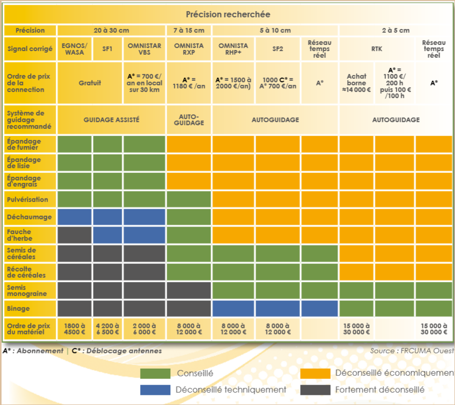
Figure 6. Which positioning technology for a given cultural route? Source: FRCUMA West.
It should be noted that these crop itineraries, if carried out with very precise positioning tools (one thinks for example of strip-till seeding techniques in soil conservation agriculture or mechanical hoeing), can also be modulated in space and time (one can for example modulate the sowing density in an agricultural plot) – this is known as intra-plot modulation.
In addition to the fairly conventional crop routes listed in this table, let us not forget the possible applications that may be more transverse (not always requiring very high precision):
- Traceability of crop operations (example of Picore to ensure that the spraying has been carried out correctly)
- Trajectory synchronization between several machines
- Certification of the origin of agricultural products
- …
Elements of conclusion
The aim of the blog was to go back over all the geolocation tools and methods in order to understand how they work and their interest for the agricultural sector. Even if the article was very oriented on satellite positioning, don’t forget that in some cases, one can sometimes position oneself very precisely in agriculture without a satellite! Think of row sensors that will allow you to guide an agricultural machine between rows of crops, of branded takeover systems that will be able to relocate in a furrow or tunnel, or even camera/sensor systems (photoelectric, light, lasers)! All these systems, depending on the case studies of the profession, may prove to be a very good alternative to a poor reception of a positioning signal, may be less expensive, or serve other applications than simple positioning.
If certain crop routes and agricultural applications can clearly benefit from ultra-precise geopositioning, this is far from always being the case. This need for precision in geo-localisation must also be reasoned according to the farmer’s unit of work. Why give agronomic information on a centimetric or even metric scale if the farmer does not think on this spatial scale, or even if the available agricultural machinery is not capable of taking this precision into account. Intra-plot modulation is a striking example of this for me. Modulating a field in a few large production areas with the help of a smartphone, or even a piece of paper attached to the window of a tractor, can already make it possible to do a very good job. Too much precision kills precision…
And finally, we must not forget that geo-positioning is all well and good, but that in order to precisely locate an object on the surface of the earth, you must not use the wrong geodetic system! I invite you to check out one of the previous posts to refresh your memory.
Some diagrams and summary graphs
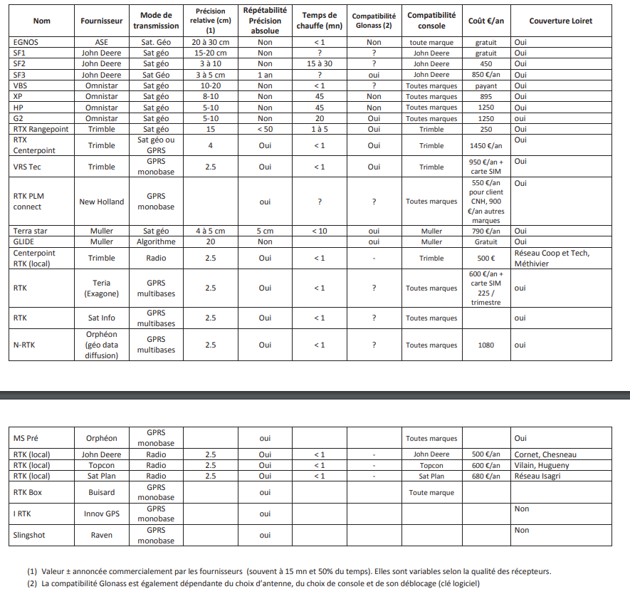
Figure 7. Classification of positioning signals. Source: Chamber of Agriculture of the Loire Valley
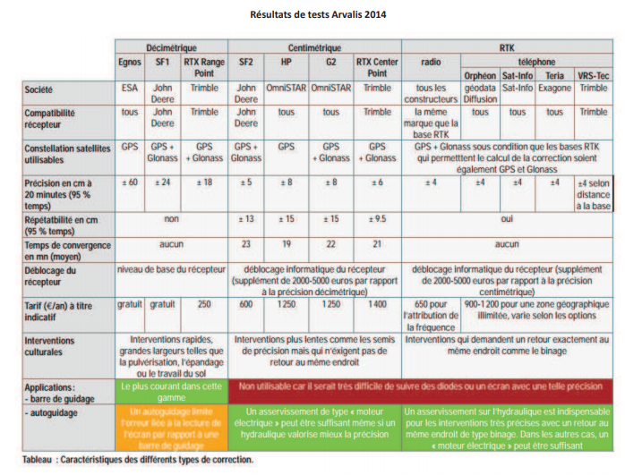
Figure 8. Experimental results around positioning signals. Source: Arvalis
Some interesting references
- Chassagne (2012), Géodésie. Le futur de la navigation par satellites : une précision à un centimètre avec le PPP. Revue XYZ, 132.
- Cilla, S. (2019). GNSS and EGNOS for farming : all you need to know from this European free service. European Conference on Precision Agriculture (Keynote Speaker). Institut Agro
- Desbourdes, C. (2010). Guidage et autoguidage RTK : un panel de solutions pour une plus grande précision. Perspectives Agricoles, 370 (https://www.perspectives-agricoles.com/file/galleryelement/pj/f7/72/70/f8/370_2787406583296596256.pdf
- Desbourdes, C. (2015). Agriculture de Précision. Communications Arvalis : https://www.evenements-arvalis.fr/reunion-agriculteurs-le-8-decembre-2015-saint-jean-de-linieres-49–@/_plugins/WMS_BO_Gallery/page/getElementStream.html?id=36446&prop=file
- Deseau, S. (2016). Choisir une correction GPS. Chambre d’Agriculture Val de Loire : https://centre-valdeloire.chambres-agriculture.fr/fileadmin/user_upload/Centre-Val-de-Loire/122_Inst-Centre-Val-de-Loire/Produire_Innover/Machinisme/45_FCC-correctionGPS_12-2016.pdf
- European Global Navigation Satellite Systems Agency (2019). PPP-RTK market and technology report (https://www.gsa.europa.eu/sites/default/files/calls_for_proposals/rd.03_-_ppp-rtk_market_and_technology_report.pdf)
- Guo, J. et al. (2018). Multi-GNSS precise point positioning for precision agriculture. Precision Agriculture
- Lahaye, R. and Ladet, S. (2014). Les principes de positionnement par satellite : GNSS. Cahier des charges techniques de l’INRAE.
- Laurichesse and Banville, (2018). Innovation: Instantaneous centimeter-level multi-frequency precise point positioning. GPSWorld. https://www.gpsworld.com/innovation-instantaneous-centimeter-level-multi-frequency-precise-point-positioning/
- Séminaire Géolocalisation en Agriculture (2018). Chaire AgroTIC. Institut Agro.
Support Aspexit’s blog posts on TIPEEE
A small donation to continue to offer quality content and to always share and popularize knowledge =) ?
2 thoughts on “Geo-positioning in agriculture”