
Few will tell you that their data is all pretty and clean and can be used as is in decision models… That’s a fact. When a dataset is collected, no one is immune to the risk of biased or outliers coming up and disrupting the quality of the data. And there are plenty of sources of error! Sensor malfunction, operator lacking of expertise … In this article, we will try to make friends with outliers data, to see in a little more detail what they look like and how to characterize them. All this in order to be able to deal with it later (but that, you shouldn’t tell them!). Come on, let’s do it.
Outliers, introduce yourself !
An anomaly or outlier can be described as an observation that deviates so far from the rest of the observations that it can be suspected that it was produced by a different mechanism (Hawkins, 1980). These outliers can be attributed to quantities of processes, for example, to a measurement error or to specific phenomena, for example, the occurrence of a fire or a climatic event (Chandola et al., 2009). The detection of outliers is one of the main areas of investigation in the Data Mining community. The identification of outliers has been extended to many applications such as fraud detection, traffic networks or military surveillance. For example, in the case of within-field yield data (which was the subject of my thesis), it has been demonstrated several times how outliers – even in limited quantities – could affect the quality of an entire dataset (Griffin et al., 2008; Taylor et al., 2007). Interestingly, depending on the field of application, some will seek to remove outliers from their datasets (because they will affect their quality and relevance) while others may, on the contrary, have a particular interest in finding and detecting outliers to highlight a phenomenon (a sharp rise in temperatures may, for example, indicate an emerging fire).
Outliers can be described in several ways: (i) local or global outliers, (ii) point, contextual or regional outliers, and (iii) univariate or multivariate outliers. Global outliers are the simplest typologies to identify. These are often data that have a very specific behaviour, very different from that of the entire dataset, i.e. these outliers are always far from the general distribution of the dataset. Local outliers are more deeply rooted in datasets. Their behaviour is not atypical in relation to the entire distribution, which does not allow for simple identification. However, these outliers are suspect with respect to their neighbouring observations (Chandola et al., 2009). Detecting these outliers requires defining neighbourhood relationships between the data in order to limit the search to a subset of neighbours rather than to the data as a whole. For non-spatialized observations (not spatially located), the neighbourhood relationships between observations depend on the proximity of non-spatial attributes. For spatial data, these neighbourhood relationships depend on the spatial proximity of an observation to its neighbours (Cai et al., 2013; Chawla and Sun, 2005). Figure 1 shows the behaviour of local and global outliers in a spatialized dataset (on the left, we look at non-spatial attributes, and on the right, we look at the relationships between observations in space with their coordinates). Four types of observations can be distinguished:
- Outlier local but not global (triangle and circle filled)
- Outlier global but not local (square filled)
- Local and global Outlier (diamond filled)
- It is not a local or global outlier
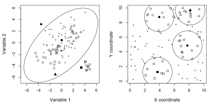
Figure 1. Local and global Outliers (after Filzmoser et al., 2014).
Punctual outliers, as one can image, are observations that have a unique and suspicious behaviour in relation to their surroundings or the entire dataset (Chandola et al., 2009). Contextual outliers are abnormal values in one specific context but not in another (Gao et al., 2010; Song et al., 2007). For example, a temperature of 30° is often not an outlier in summer, but it can be considered as such in winter. Finally, regional outliers are a subset of closely related observations – in space or not – that share common suspicious characteristics with respect to their vicinity or the remaining dataset (Zhao et al., 2003). The final distinction that can be made concerns the univariate or multivariate aspect of these outliers (Chandola et al., 2009). In the first case, the dataset consists of only one attribute and an outlier is defined as a suspicious observation with respect to that attribute (Cousineau and Chartier, 2010; Rousseeuw and Hubert, 2011). In the multivariate case, the situation becomes more complex because an outlier may present a normal behaviour from the point of view of a particular attribute, but may have a truly specific behaviour according to another attribute (Ernst and Haesbroeck, 2013; Filzmoser et al., 2014; Filzmoser, 2014). The challenge is the diversity of configurations within a multivariate data set.
The three approaches that have been introduced to define the key concepts of outliers are obviously linked! It is possible to observe a multivariate local outlier value or a univariate global or regional outlier value.
A brief overview of outlier detection methods
Given the many fields of application that involve the detection of aberrant observations, the literature offers a considerable number of approaches to outlier detection (Kou, 2006; Sun, 2006). In general, outlier detection techniques can be classified into 7 major groups, each based on (i) distribution, (ii) density, (iii) distance (iv) depth, (v) classification, (vi) aggregation, and (vii) spectral decomposition or data projection. I will quickly introduce you to these large families with examples of associated methods in square brackets. For motivated and interested readers, a large part of the references is available at the end of the post!
- Distribution-based[Gaussian mixing models, Bayesian approach, nucleus estimation…] : These methods aim to model the distribution of data with a known or unknown function, i.e. a parametric or non-parametric approach (Hawkins, 1980). Observations whose behaviour is suspect in relation to established distributions are considered outliers (Chhabra et al., 2008; Ngan et al., 2016). Thresholds are often set to decide whether a value differs significantly from the distribution. Parametric methods are often criticized because the distribution of data is usually unknown in advance.
- Density-based[LOF, LOCI, LoOp…]: These approaches assume that the density of observations near an outlier is significantly lower than the density of observations near an expected or true value (Breunig et al., 2000; Goldstein, 2012; Kriegel et al, 2009; Papadimitriou et al, 2003; Tang et al., 2002). These techniques are sometimes preferred to distance-based methods when the dataset is composed of subsets of varying densities. Thresholds are set to determine the proximity of an observation and the limit beyond which a value is considered abnormal.
- Distance-based[SLOM, ROF…]: This approach uses the distance between an observation and the dataset to assess whether or not the observation is an outlier (Cai and He, 2010; Chawla and Sun, 2005; Dang et al, 2015; Fan et al, 2006; Filzmoser et al, 2014; Filzmoser, 2014; Harris et al, 2014). Euclidean and Mahalanobi distances are often reported in these methods. Several authors have shown that current estimates of the location and scale of a data set, i.e., mean and variance, are strongly influenced by outliers. More robust estimates have been developed to make distance-based methods more reliable (Rousseeuw and Hubert, 2011). The thresholds are similar to those of density-based methods.
- Depth-based[KSD…] : The data set is modeled by a set of convex hulls whose objective is to group the data according to their proximity to the core of the data set (Chen et al., 2009). Convex hulls near the core of the data set contain the most expected values while outer hulls discriminate against outliers. Calculation time becomes excessive when the dimensions of the data set exceed 3 or 4 (Papadimitriou et al., 2003).
- Classification-based[SVM, Bayesian approach…]: Classification-based methods may or may not be supervised (Yang et al., 2010). In the first case, a training dataset for which the position of outliers is known is used to construct a classifier that will distinguish outliers in a validation data set. In the second case, the classifier tries to model the data set without using a test or a validation data set.
- Clustering-based[CLARANS, DBSCAN…]: These approaches seek to group observations into different subsets and consider outliers to be process residues, i.e. observations that are not attached to any subset (Chawla and Gionis, 2013; Muller et al., 2012). Intuitively, the last observations to be attached are more likely to be outliers. These methods are sometimes criticized because their output depends heavily on the choice of the clustering algorithm. In addition, since these approaches were initially designed primarily for data clustering, their potential for detecting outliers could be questioned (Gao et al., 2010; Kou, 2006).
- Spectral decomposition-based[PCA, GWPCA…]: Observations are projected onto a new sub-space to facilitate the detection of outliers (Demšar et al. 2013 ; Filzmoser et al., 2007 ; Harris et al., 2014). This approach is preferred when the data set has multiple dimensions, i.e., when other methods would not produce a result within a reasonable time (Fritsch et al., 2011; Sun, 2006). These techniques provide a solution to the so-called curse of dimensionality problem (“Curse of dimensionality”, Schubert, 2013; Sun, 2006). This problem is due to the fact that by increasing the number of data dimensions (the number of variables that characterize them), outliers will be more and more rooted in the dataset and will be more and more difficult to detect. The number of main components to choose for decomposition remains a challenge and is always defined by a threshold.
In the literature, methods based on distance, density and clustering are most often mentioned. Hybrid approaches, i. e. combining several of these techniques, have been proposed by several authors (Harris et al., 2014; Mendez and Labrador, 2013).
Outliers are generally identified in two ways, i.e., by labelling or scoring (Kriegel et al., 2009). Outliers can be labelled – labelling – which means that at the end of the process, a binary classification is obtained, i.e. the observation is either considered outlier or non-aberrant. Other methods associate a degree of outlierness to the data (scoring) which enables to obtain a ranked list of outliers (Muller et al., 2012; Papadimitriou et al., 2003). Note that by setting a threshold for scoring approaches, a binary classification is obtained as if the data had been labelled. Rating/Scoring methods are generally preferred because they allow for a more in-depth study of the origin and involvement of outliers in data sets.
In this section, the main focus has been on detection methods, i.e., trying to search for and find outliers. We could imagine solving the problem differently by trying to smooth the data and therefore limit the influence of our little outliers! This is what happens quite well in the field of signal processing. I will not go into the details of this type of approach but here are some examples if you want to find out more:
- Average and median filters,
- Savitsky-Golay filter,
- Transformed from Fourier,
- Wiener and Kalman filters,
- Spectral subtraction,
- Transformed into wavelets,
- Hilbert-Huang Transform[Empirical decomposition mode]
- …
How to judge the quality of a detection method?
The ultimate objective of outlier detection methods is to identify outliers as well as possible and without confusion. The authors focus on reducing the number of swamping effects, i.e. avoiding misclassifying an accurate observation as an outlier. Some approaches also consider the complementary error to the first one (masking effect) in which outliers are not identified as such; these observations are classified as false negatives (Ben-gal, 2005; Kou, 2006). Characterization of these two types of errors obviously requires knowing in advance where outliers are in the dataset, which is generally not the case. As a result, these methods are often first validated on synthetic or artificial datasets (in which outliers are voluntarily added) and then applied to real datasets. At the end of the processing operation, several criteria can be analysed to assess the relevance of the proposed methods. Studies generally report false positives and false negatives rates (Chandola et al., 2009). The authors also estimate the performance of their classifier using the ROC curve – a graph showing the ratio between true positives and false negatives rates (Kriegel et al., 2009; Zhang et al., 2010). Improved signal-to-noise ratio (SNR) is often a good quality criterion for single and multidimensional signals. The lower the ratio, the more powerful the filtering method is.
Finally, the computation time of algorithms must be seriously taken into account. With increasingly resolute and accurate acquisition systems, and with the storage of large amounts of data, the efficiency of classifiers is a central issue. Very often, studies that propose general techniques for detecting outliers address this specific point (Jin et al., 2006; Shekkar et al., 2003; Sun, 2006). The authors determine the effectiveness of each of their processing steps in order to evaluate the scalability of their methods to larger and higher-dimensionality datasets.
What to do once outliers are detected?
This issue is indeed a major concern after the identification of outliers. In the case of signal processing, which I mentioned briefly (when unidimensional or multidimensional signals are smoothed), the question is no longer too relevant because the objective is not to detect outliers but rather to smooth the observations. When outliers are identified, two scenarios are possible: outliers can be deleted or corrected. The elimination of outliers is brutal but instantaneous. However, the size of the dataset can be significantly reduced if there is a large amount of outliers. It is also questionable if outlier detection methods are not robust. For example, if the false positive rate is significant, i.e. an object is incorrectly identified as an outlier, deleting outliers will result in the deletion of relevant observations. The correction of an outlier is a more complex problem. It is indeed possible to use the vicinity of an observation or some general patterns/trends in the data to modify the value of an outlier, but these methods are likely to add noise to the data sets if this work is not done with great care. One possible correction would be to replace an outlier with the result of interpolation from neighboring objects. But at that moment we take the risk of smoothing the information in our dataset, one must be aware of this….
Disadvantages and limitations of current methods: general application and automation
Most of the detection methods described above use manual thresholds for data filtering. However, is it really conceivable to apply similar thresholds to two sets of data that have been acquired under particularly different conditions? How can a large number of datasets be processed quickly if it is necessary to manually determine new thresholds for each new dataset?
All the outlier detection methods that have been presented require thresholds at different levels to identify outliers. The choice of these thresholds can have a significant impact on the detection of abnormal values. For example, one of the first thresholds to be set relates to the establishment of a neighbourhood for each observation (Breunig et al., 2000; Knorr et al., 1998). This threshold often corresponds to a distance to the kth neighbor or a distance that ensures that k neighbors belong to the neighborhood of an observation. In scoring approaches, the threshold above which an observation is considered outlier is crucial. A low threshold would increase the false negative rate while a high threshold would increase the false positive rate. From a general point of view, the interpretation of scores is a relatively complex task for non-specialists. These scores are often very different from one method to another and can have completely different meanings. Some authors have tried to simplify these scores by scaling them between 0 and 1 so that they can be understood in a probabilistic approach, simpler to handle; a value of 1 indicating that an object has a 100% chance of being considered an outlier (Kriegel et al., 2009). Even if the method is more practical, setting a threshold between 0 and 1 remains difficult and subject to expertise.
It can also be added that most of the reported filtering methods must be applied under specific conditions. Several signal processing approaches require that input signals be linear or stationary. Some outlier detection methods are limited a priori by distributions or type of input data. In order to develop very general and automated tools, these prerequisites are a real obstacle. It is an obstacle that prevents some methods from being used on multiple and diverse data. Of course, general methods are less powerful than specific methods, but they can be used a little more widely.
References
Ben-gal, I. (2005). Outlier detection, 1–16.
Breunig, M. M., Kriegel, H.-P., Ng, R. T., & Sander, J. (2000). LOF: Identifying Density-Based Local Outliers. Proceedings of the 2000 Acm Sigmod International Conference on Management of Data, 1–12. http://doi.org/10.1145/335191.335388
Cai, Q., & He, H. (2010). IterativeSOMSO : An iterative self-organizing map for spatial outlier detection. Theoretical Computer Science, (March). http://doi.org/10.1007/978-3-642-13318-3
Cai, Q., He, H., & Man, H. (2013). Spatial outlier detection based on iterative self-organizing learning model. Neurocomputing, 117, 161–172. http://doi.org/10.1016/j.neucom.2013.02.007
Chandola, V., Banerjee, A., & Kumar, V. (2009). Outlier Detection : A Survey.
Chawla, S., & Gionis, A. (2013). k -means– : A unified approach to clustering and outlier detection.
Chawla, S., & Sun, P. (2005). SLOM: A new measure for local spatial outliers. Knowledge and Information Systems, 9(4), 412–429. http://doi.org/10.1007/s10115-005-0200-2
Chen, Y., Dang, X., Peng, H., & Bart, H. L. (2009). Outlier detection with the kernelized spatial depth function. IEEE Transactions on Pattern Analysis and Machine Intelligence, 31(2), 288–305. http://doi.org/10.1109/TPAMI.2008.72
Chhabra, P., Scott, C., Kolaczyk, E. D., & Crovella, M. (2008). Distributed spatial anomaly detection. Proceedings – IEEE INFOCOM, 2378–2386. http://doi.org/10.1109/INFOCOM.2007.232
Cousineau, D., & Chartier, S. (2010). Outliers detection and treatment : a review . Internation Journal of Psychological Research, 3(1), 58–67.
Dang, T., Ngan, H. Y. T., & Liu, W. (2015). Distance-Based k -Nearest Neighbors Outlier Detection Method in Large-Scale Traffic Data, (February 2016). http://doi.org/10.1109/ICDSP.2015.7251924
Ernst, M. and Haesbroeck, G. (2013). Robust detection techniques for multivariate spatial data. Poster.
Fan, H., Zaïane, O. R., Foss, A., & Wu, J. (2006). A nonparametric outlier detection for effectively discovering top-N outliers from engineering data. Lecture Notes in Computer Science (including Subseries Lecture Notes in Artificial Intelligence and Lecture Notes in Bioinformatics), 3918 LNAI, 557–566. http://doi.org/10.1007/11731139_66
Filzmoser, P. (2004). A multivariate outlier detection method. Seventh International Conference on Computer Data Analysis and Modeling, 1(1989), 18–22. Retrieved from http://computerwranglers.com/com531/handouts/mahalanobis.pdf
Filzmoser, P., Maronna, R., & Werner, M. (2007). Outlier identification in high dimensions. Filzmoser, P. Maronna, R. Werner, M. http://doi.org/10.1016/j.csda.2007.05.018
Filzmoser, P., Ruiz-gazen, A., & Thomas-agnan, C. (2014). Identification of local multivariate outliers.
Fritsch, V., Varoquaux, G., Thyreau, B., Poline, J.-B., & Thirion, B. (2011). Detecting Outlying Subjects in High-Dimensional Neuroimaging Datasets with Regularized Minimum Covariance Determinant. Medical Image Computing and Computer-Assisted Intervention, Miccai 2011, Pt Iii, 6893, 264–271. Retrieved from <Go to ISI>://WOS:000306990200033
Gao, J., Liang, F., Fan, W., Wang, C., Sun, Y., & Han, J. (2010). On community outliers and their efficient detection in information networks. Proceedings of the 16th ACM SIGKDD International Conference on Knowledge Discovery and Data Mining (KDD ’10), 813–822. http://doi.org/10.1145/1835804.1835907
Goldstein, M. (2012). FastLOF: An Expectation-Maximization based Local Outlier detection algorithm, (1), 2282–2285.
Griffin, T., Dobbins, C., Vyn, T., Florax, R., & Lowenberg-DeBoer, J. (2008). Spatial analysis of yield monitor data: case studies of on-farm trials and farm management decision making. Precision Agriculture, 9(5), 269–283. http://doi.org/10.1007/s11119-008-9072-2
Harris, P., Brunsdon, C., Charlton, M., Juggins, S., & Clarke, A. (2014). Multivariate Spatial Outlier Detection Using Robust Geographically Weighted Methods. Math Geosciences, 1–31. http://doi.org/10.1007/s11004-013-9491-0
Jin, W., Tung, A. K. H., Han, J., & Wang, W. (2006). Ranking outliers using symmetric neighborhood relationship. Lecture Notes in Computer Science (including Subseries Lecture Notes in Artificial Intelligence and Lecture Notes in Bioinformatics), 3918 LNAI, 577–593. http://doi.org/10.1007/11731139_68
Knorr, E. M., & Ng, R. T. (1998). Algorithms for Mining Datasets Outliers in Large Datasets. Proceedings of the 24th VLDB Conference, New York, USA.
Kou, Y. (2006). Abnormal Pattern Recognition in Spatial Data.
Kou, Y., Lu, C., & Chen, D. (2006). Spatial Weighted Outlier Detection. In Proceedings of SIAM Conference on Data Mining, 613–617. http://doi.org/10.1137/1.9781611972764.71
Kriegel, H., Kröger, P., Schubert, E., & Zimek, A. (2009). LoOP : Local Outlier Probabilities. Proceeding of the 18th ACM Conference on Information and Knowledge Management – CIKM ’09, 1649. http://doi.org/10.1145/1645953.1646195
Lu, C.-T., Chen, D., & Kou, Y. (2003). Algorithms for spatial outlier detection. Third IEEE International Conference on Data Mining, 0–3. http://doi.org/10.1109/ICDM.2003.1250986
Mendez, D., & Labrador, M. A. (2013). On Sensor Data Verification for Participatory Sensing Systems. Journal of Networks, 8(3), 576–587. http://doi.org/10.4304/jnw.8.3.576-587
Muller, E., Assent, I., Iglesias, P., Mulle, Y., & Bohm, K. (2012). Outlier Ranking via Subspace Analysis in Multiple Views of the Data.
Ngan, H. Y. T., Lam, P., & Yung, N. H. C. (2016). Outlier Detection In Large-scale Traffic Data By Naïve Bayes Method and Gaussian Mixture Model Method, (February).
Papadimitriou, S., Kitagawa, H., Gibbons, P. B., & Faloutsos, C. (2003). LOCI: fast outlier detection using the local correlation integral. Proceedings 19th International Conference on Data Engineering (Cat. No.03CH37405), 315–326. http://doi.org/10.1109/ICDE.2003.1260802
Rousseeuw, P. J., & Hubert, M. (2011). Robust statistics for outlier detection. Wiley Interdisciplinary Reviews: Data Mining and Knowledge Discovery, 1(1), 73–79. http://doi.org/10.1002/widm.2
Schubert, E. (2013). Generalized and efficient outlier detection for spatial, temporal, and high-dimensional data mining. Retrieved from http://nbn-resolving.de/urn:nbn:de:bvb:19-166938
Song, X., Wu, M., Jermaine, C., & Ranka, S. (2007). Conditional Anomaly Detection. IEEE Transactions on Knowledge and Data Engineering, (0325459), 1–14.
Sun, P. (2006). Outlier Detection in High Dimensional , Spatial and Sequential Data Sets.
Taylor, J. A., Mcbratney, A. B., & Whelan, B. M. (2007). Establishing Management Classes for Broadacre Agricultural Production. Agronomy Journal, 1366–1376. http://doi.org/10.2134/agronj2007.0070
Zhang, Y., Meratnia, N., & Havinga, P. (2010). Outlier Detection Techniques for Wireless Sensor Networks: A Survey. IEEE Communications Surveys & Tutorials, 12(2), 1–12. http://doi.org/10.1109/SURV.2010.021510.00088
Zhao, J., Lu, C., & Kou, Y. (2003). Detecting Region Outliers in Meteorological Data, 49–55.
Support Aspexit’s blog posts on TIPEEE
A small donation to continue to offer quality content and to always share and popularize knowledge =) ?