
Precision agriculture tools (pedestrian, static, tractor-mounted or airborne sensors, etc.) make it possible to acquire agronomic and environmental data sets at impressive spatial, temporal and attribute resolutions. Generally speaking, we tend to trust these captured data (sometimes too much), i.e., we often use them as they are, without really asking ourselves too many questions! However, these data are often subject to uncertainty, and it is important to pay attention to it! Whatever the uncertainties, the most important thing when analyzing data is to be able to list, characterize and quantify the uncertainties, so as to clarify the confidence we will be able to place in the data before making our final decision.
Different sources of uncertainty
Quite simply, uncertainties can be classified into two main categories:
– Non-random (epistemic) uncertainties: These are the uncertainties that can be considered to be in hand or that could be reduced, for example if there was a better knowledge of the systems/crops being studied, if more accurate and/or calibrated sensors were available, or if more robust and reliable procedures were used
And we can find many examples: poorly calibrated yield sensor (uncertainty on the yield attribute value that is given by the sensor), unreliable GNSS receiver (uncertainty on the spatial positioning of a measurement from an on-board sensor), few soil samples (uncertainty on the representativeness of field-scale measurements), productivity areas expertly delimited by a farmer or advisor (uncertainty on the exact boundaries/borders of the areas), not exactly perfect agronomic model [it is impossible anyway] (uncertainty on model outputs)…
– Random (natural) uncertainties: On the contrary, those are the uncertainties that cannot be reduced because they are the consequences of processes that we cannot control
Once again, some examples in precision agriculture: the volatility of the purchase price of inputs or the selling price of a cereal crop (uncertainty about the turnover, fixed and variable costs of the farm), medium/long term climatic conditions (uncertainty about the impact of a decision at a time “t1” on the result at a time “t2”), the intrinsic or natural variability of plants (uncertainty about the value of an agronomic parameter of a plant when this same parameter is measured very precisely on a plant extremely close in space).
Uncertainty analysis
All the data we collect will generally be integrated and compiled into a model (whether expert, mathematical or whatever) that will lead to decision making. When we talk about uncertainty analysis, we are actually trying to know the uncertainty of our model output variable. For example, if I am a grain farmer, my sales are uncertain (because there are many uncertainties as we saw earlier) but I would still like to have an idea of the likely distribution of my sales. To have this distribution, I must therefore take into account all the data necessary to calculate my sales (my input data) and the associated uncertainties. So at some point in time, I will have to model these uncertainties so that I can take them into account in a slightly more objective way. Without going into detail, we can imagine several modelling approaches.
The first, very simple, is to reason by scenario. This is an approach that we can imagine when we don’t really have an idea about the level of uncertainty to take into account for our data of interest (in the context of random variability for example). The approach therefore consists in proposing several possible scenarios (we have not made much progress…) for the input data we are trying to evaluate. Let us take the example of the “cereal price” input data and its associated uncertainty, the “price volatility”. I can imagine a first scenario where I would sell my wheat at 150€ per tonne, and a second scenario where I would sell it at 200€ per tonne. Punctual scenarios are used here. I can therefore very well imagine a worst-case scenario (very low price per tonne) or an advantageous scenario (very high price per tonne) to assess the uncertainty of my turnover. I can also go further by imagining an average scenario, which would take into account the average price of wheat over 10 years.
The second approach, a little more advanced, is to reason in a probabilistic way. The idea here is to propose continuous probability scenarios for the data being evaluated. But this approach requires us to have a little more insight into the head of our uncertainty. On the same example as before, if I know the history of wheat prices over 20 years, I can construct a probability law of wheat prices and therefore highlight the fact that some scenarios are more likely than others.
To evaluate the likely distribution of my sales, I will therefore be able to calculate a lot of different sales figures using, for each iteration, a wheat price whose value will have been derived from the scenarios or the probability law that I would have put in place (several tools exist to draw in these probability laws, for example the Monte Carlo method). At the end of my iterations, I will therefore have a distribution (which I can try to model or approximate if I want) that will show me the variability of my output variable (my sales) according to my input variable (wheat price). We will therefore have completed the uncertainty analysis of our revenue. The example taken here is very simplified because we only looked at one input variable but it is totally extensible to a large number of input variables. However, there are some precautions to take when starting to work on uncertainty (whether on one or more variables), especially for notions of correlations between individuals or variables.
Knowing the uncertainty associated with our output variable is certainly interesting. But it is still more relevant to know the input parameters that will have the major influence on this output variable. It is true that if an input parameter has little influence on the output variable (and therefore its uncertainty), there is not much interest in spending considerable time on it. This is what we will see in the next section with the sensitivity analysis!
A focus on sensitivity analysis
The purpose of sensitivity analysis is to assess the importance of a model’s input parameters on the output interest variables of that model. This will allow us to look at the parameters on which to focus to reduce the uncertainty associated with our output variable. Sensitivity analysis makes it possible to answer questions such as: What are the most impactful input parameters of my model? How much of the variability of my model is explained by the input parameter X? How does the variability of a model’s input data affect the variability of the model’s output response?
Sensitivity analysis methods are mainly of three types:
– The so-called “screening” methods (e.g. Morris) seek to evaluate the influence of the input parameters of a model, by varying these parameters one by one (Morris is part of the so-called OAT, One At a Time methods). These methods are adapted when there are many input parameters because they allow the influence parameters to emerge more quickly than the so-called “global” methods, which are very demanding in terms of computation time.
– The so-called “local” methods seek to assess the extent to which a small variation in the values of an input parameter of a model influences the outputs of that model. These methods are local because they are not interested in all the possible values that the input parameter can take, but only in local variations around a target value,
– Global” methods, on the other hand, focus on the variability of the model’s output over its entire range of variation. The most commonly used methods (Sobol and Fast methods), use a variance decomposition approach to represent the proportion of model variability explained by an input or input group of the model
Example :
Recently, I have been working on the sensitivity analysis of a fertilizer recommendation model to its input parameters (in particular in relation to soil sample analyses in the laboratory, the interpretation of these soil analyses in expert classes, the agricultural practices carried out and/or planned or the past production level and the production objective of the future crop). In this study, the sensitivity analysis was performed using the Sobol global method for several reasons. Since the model used some qualitative data (e.g. fertilization strategy, future of crop residues, etc.), I chose to use global methods because “local” methods could not be applied (studying local variations of a non-continuous variable did not really make sense) and “Morris” screening methods were not very suitable either. Sobol’s methods, for their part, are interesting for several reasons. First of all, they make it possible to free oneself from this previous constraint on qualitative variables. Second, these methods generate easily interpretable indices (the Sobol indices) to express the proportion of model variance explained by the input variables. Finally, Sobol’s methods make it possible to characterize not only the impact of a single parameter on the model but also the interactions between this parameter and the remaining parameters. For example, it is quite possible that a single parameter may not be of much importance, but that it is its interaction with other input parameters of the model that makes it interesting (Figure 1)
One of the important assumptions to be made in order not to bias the results of a sensitivity analysis is to ensure that the input variables of the model are not correlated with each other. It has to be said that some of the parameters of the model were! This was the case, for example, between the crop species and their yield (two different species may not have the same yield level) or between a soil type and its initial P/K content (some soil types will always have a lower P/K content than other soil types). To limit the correlation effects between variables, sensitivity analyses were carried out by soil type and crop.
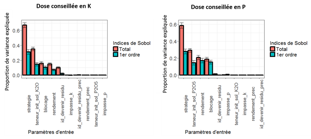
Figure 1. Sensitivity analysis of a fertilizer recommandation model.
Uncertainty and sensitivity analyses are very powerful tools to characterize and clarify the agronomic models we use. They are also relevant methods when deploying a model at an operational level, particularly because they allow efforts to be focused on the really important parameters of the model and thus facilitate its wider use. In wanting to work with ever more precise approaches (whether at a spatial or temporal level), it is necessary to be interested in the quality of the data we use and therefore, consequently, in their uncertainty.
Support Aspexit’s blog posts on TIPEEE
A small donation to continue to offer quality content and to always share and popularize knowledge =) ?