
Computing an experimental variogram
The usefulness of variograms in Precision Agriculture studies have been largely detailed in a previous post. This is effectively a valuable tool to study the spatial structure of agronomic and environmental spatial datasets. This post will make use of a dataset that was created following the methodology of the post : “Simulating spatial datasets with known variability”. This dataset is a dataframe (a table) with three columns: the longitude (x), the latitude (y) and the variable of interest (RDT, the yield production in tons per hectare).
## Load the packages of interest
library(gstat)
library(sp)

head(RDT_gaussian_field)
  x y      RDT
1 1 1 7.788309
2 2 1 7.692076
3 3 1 8.433189
4 4 1 8.147506
5 5 1 9.124606
6 6 1 8.733661


class(RDT_gaussian_field)
[1] "data.frame"

## Transform the dataframe into a SpatialPointDataFrame
## The objective is to obtain a spatial object
coordinates(RDT_gaussian_field)=~x+y

class(RDT_gaussian_field)
[1] "SpatialPointsDataFrame"
attr(,"package")
[1] "sp"

## If the coordinates are not projected (ex : if they are in degrees), there is a need to reproject the observations first.
## Here it is unnecessary because observations are located on a regular grid
## Computation of the variogram
Vario_RDT=variogram(RDT~1, ## Here, we assume that there is a constant trend in the data.
                           ## It would not have been the case for an elevation study along a hillslope where
                           ##there would have been a clear elevation trend regarding the spatial coordinates (along the hillslope)
                     data=RDT_gaussian_field)

## Plot the experimental variogram
plot(Vario_RDT)
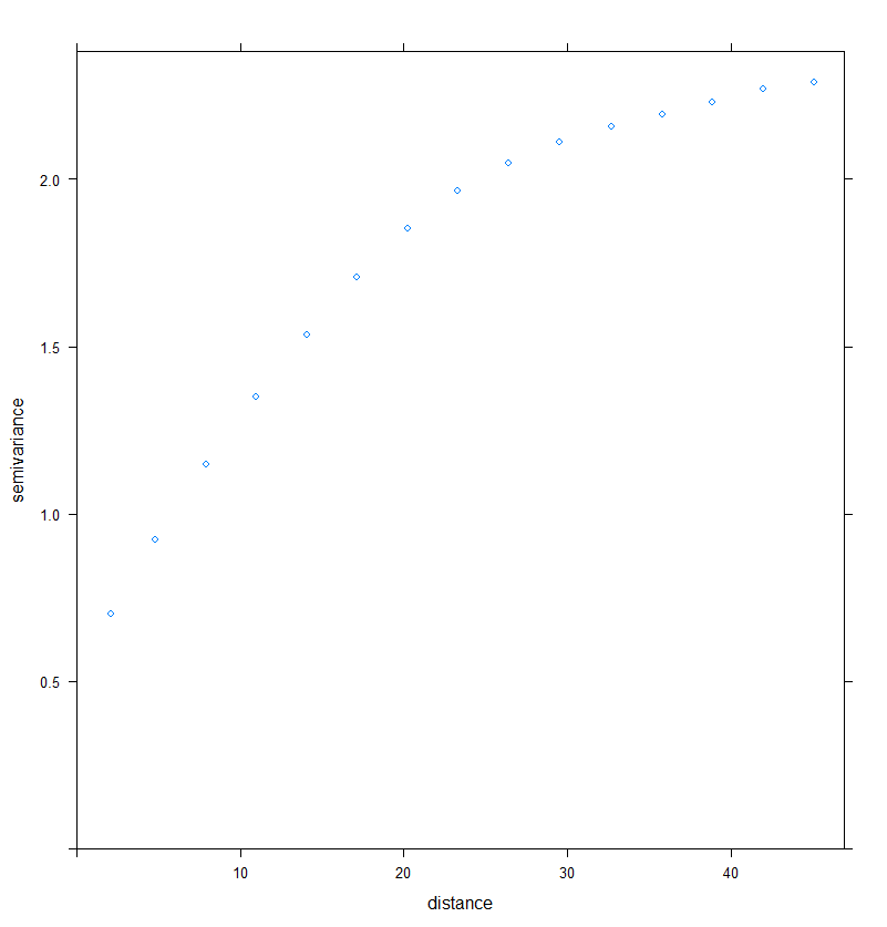
Figure 1. Implementation of the experimental variogram
Fitting a semi-variogram model to the data
Once the semi-variogram has been computed, the objective is to fit a semi-variogram model to describe the spatial structure of the observations. This can be done as follows:
## Fit a semi-variogram model
Vario_RDT.fit = fit.variogram(Vario_RDT,
                               ## A semi-variogram model needs to be manually proposed but it is only to drive the fit
                               ## The parameters will certainly be slightly changed after the fit
                               model = vgm(psill=2, ## Partial Sill (do not confound with the sill)
                                           model="Sph",  ## A Spherical model seems appropriate
                                           range=30,     ## Portée pratique = Maximal distance of autocorrelation
                                           nugget=0.5))  ## Effet pépite = Small-scale variations
## Look at the result of the fit
> Vario_RDT.fit
  model     psill    range
1   Nug 0.5610564  0.00000
2   Sph 1.6354986 33.53541
## The first estimation of the parameters was relatively good so the output is very similar to the fit
## Plot the variogram with the corresponding model
plot(Vario_RDT,Vario_RDT.fit)
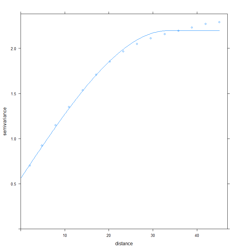
Figure 2. Fitting a semi-variogram model to the data
Looking deeper into the semi-variogram computation
The previous code snippets only intended to plot a simple variogram and fit a semi-variogram model to the observations. All the parameters of the variogram function of the ‘gstat’ package were used by default. However, in most cases, there is a need to play with these parameters to be sure that the variogram is correctly displayed. Among these settings, two are of particular interest : cutoff and width. The cutoff represents the maximal spatial distance taken into account between two observations. The width is the distance interval over which the semi-variance is calculated.
## Set the cutoff and width in the variogram function
Vario_RDT=variogram(RDT~1,data=RDT_gaussian_field,cutoff=30,width=5)
Vario_RDT=variogram(RDT~1,data=RDT_gaussian_field,cutoff=60,width=5)
Vario_RDT=variogram(RDT~1,data=RDT_gaussian_field,cutoff=90,width=10)
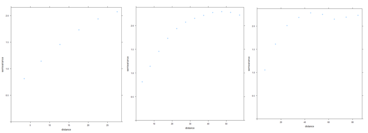
Figure 3. Influence of the parameters cutoff and width on the shape of the semi-variogram
Note that if the cutoff is set too low, some spatial structures may be missed or the global spatial structure might be misunderstood. If the width parameters is set too high, the spatial structure will be very smoothed and some useful information might be lost. Performing a semi-variogram analysis requires to carefully set the variogram parameters so that the spatial structure is well-captured.
Isotropic or anisotropic process ? Computing directional variograms
So far, the process underlying the observations was considered isotropic, that is to say not directionnaly dependent. However, sometimes, a exterior factor (ex: slope or temperature) may affect the spatial structure of the dataset. Here comes the need to compute directional variograms. The semi-variogram is computed in the same way as before except that some other parameters are added to the variogram function.
## Set the directions of interest to compute the directional variograms
RDT_vario.dir=variogram(RDT~1,
                         data=RDT_gaussian_field,
                         alpha = c(0, 45, 90, 135))
                         ## Semi-variograms will be plotted in the directions 0, 45, 90 and 135°
                         ## The variogram is a symmetric measure so for instance, the directions 45
                         ## and 225° (45+180) will lead to the same results

## Plot the directional variograms
plot(RDT_vario.dir)
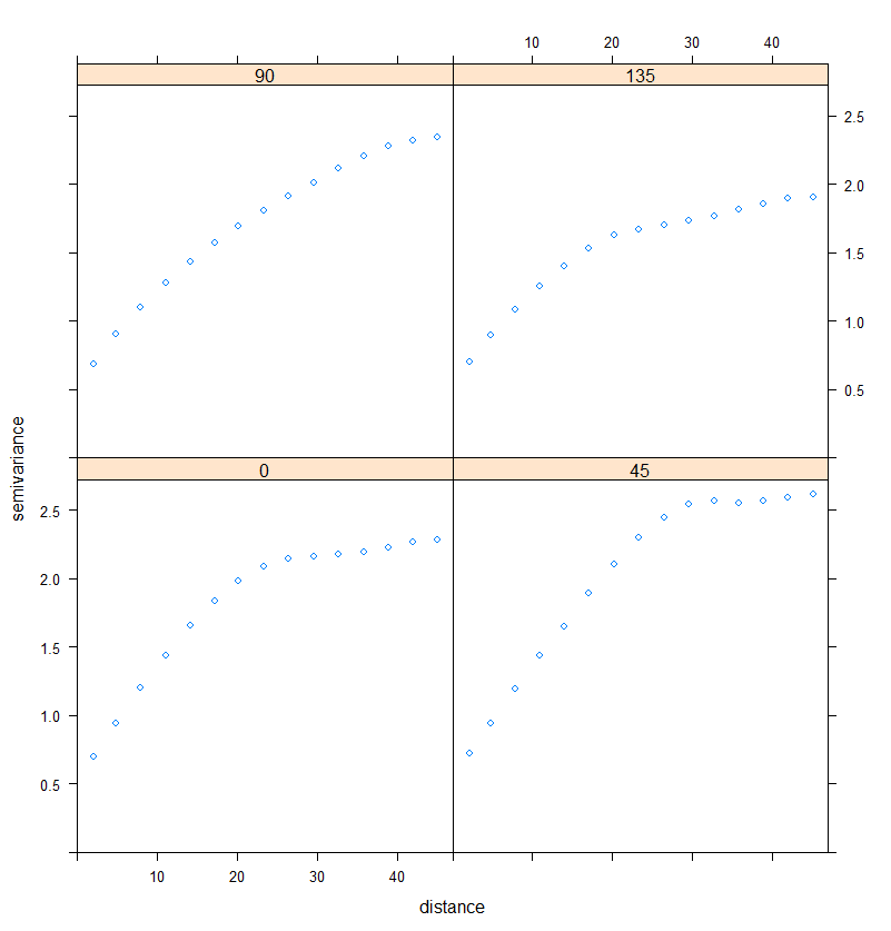
Figure 4. Directional variograms
It must be noted that the variograms are computed in the directions that were set with a certain degree of tolerance.
For instance, if the direction 45° is chosen, what to do with the pairs of observations whose direction between observations is 59° ? Should they be discarded ?
By default, the computation is averaged over the nearest direction that is set.
For instance, in the previous code snippet with the directions 0, 45, 90 and 135, the direction interval was 45°. Each directional variogram was averaged over a direction X +/- 22.5° (45 divided by 2). For example, the directional variogram at 90° considered all the directions between 67.5° and 112.5°.
This tolerance can be parametrized with the variables tol.hor (horizontal tolerance) and tol.ver (vertical tolerance) in the variogram function.
Finally, there is the possibility to fit a variogram model to the directional variograms previously computed. Note that a specific model cannot be fitted to each directional variogram at the same time. Only one model will be provided
## Fit a semi-variogram model to the directional variograms.
RDT_variodir.fit = vgm(psill=2,  ## A semi-variogram model is estimated by eye as before
                        model="Sph",
                        range=30,
                        nugget=0.5,
                        ## Set the anisotropy parameters. They also have to be estimated by eye
                        anis = c(45,  ## Direction of larger range regarding all the directional variograms
                                      ## Here, the direction 45° seems to be that of larger range
                                 0.6)) ## Ratio of the minor range (approximately 25m)
                                       ## to the maximal range (approximately 40m)

## Plot the directional variogram and associated model
plot(RDT_vario.dir, RDT_variodir.fit)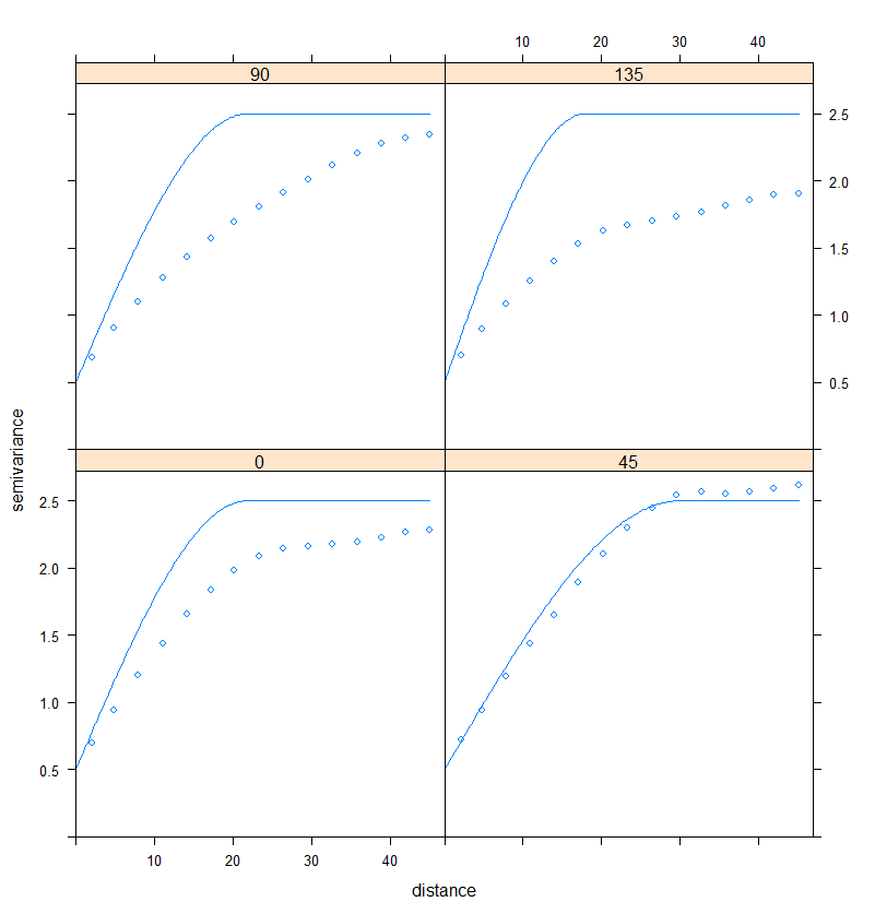
Figure 5. Fitting a semi-variogram model to the directional variograms
By looking at Figure 5, it seems that the spatial structure is relatively stronger in the 0 and 45° direction. To perform a more precise analysis, one would have to test other directions and maybe set lower tolerance angles. Directional variograms are a useful tool to spot quickly a specific direction of variation. Here, the process could be considered as isotropic because the differences are not extremely important between the directions of interest.
From all that has been said, it must be understood that manual supervision is really important when dealing with semi-variograms. I would recommend not to automate a semi-variogram analysis as it could lead to misleading conclusions. If the spatial structure is very well-defined and extremely clear, this won’t be a problem because default parameters might be used. However, in most cases, the automatic fit of a semi-variogram model might be problematic.
More information can be found in that very useful document from Edzer Pebesma
Support Aspexit’s blog posts on TIPEEE
A small donation to continue to offer quality content and to always share and popularize knowledge =) ?