
There is no such thing as a perfectly homogenous agricultural field ! And this is simply due to the fact that we work with living organisms and that we are confronted with phenomena that are all more complex than each other (soil, climate, plants, agricultural practices…), and which also have the unfortunate tendency to interact with each other. These phenomena vary both spatially (and on different scales – plot, farm, production basin, etc.) and temporally (day, week, month, etc.). We can indeed imagine very different soil zones within the same agricultural field, or a biomass that changes significantly over the course of the season. This often raises many questions about the variability or heterogeneity of these phenomena! Am I able to understand this variability? Am I able to take it into account in my tactical and strategic choices, in the short, medium or long term? Does considering this variability make sense in view of my production constraints and objectives? But first and foremost, how can I objectively measure this variability?
This short post is a synthesis of work done during my thesis: “How to measure and report within-field variability – a review of common indicators and their sensitivity” published in the journal Precision Agriculture. We will focus here on existing indicators to measure and quantify spatial heterogeneity (we will not discuss the temporal case here). Interested readers can return to read the full article.
Why use indicators of spatial variability
In the literature, we can distinguish four main use cases for which the authors use indicators of spatial variability :
- Case Study 1 (UC1): To objectively evaluate the magnitude of variation of a phenomenon. It should be noted here that we are not talking about spatial variability, but rather attributive variability (without consideration of spatial).
- Case Study 2 (UC2): To objectively assess the spatial variability of a phenomenon
- Case Study 3 (UC3): To compare the spatial structure between several agronomic attributes in the same plot, or between the same agronomic attribute but within different plots. This is a kind of spatial variability benchmark. It can be used to order plots or spatial units from the largest to the smallest spatial variability, or for example to compare the impacts of certain agricultural practices on the observed spatial variability
- Case study 4 (UC4): To create a modulation map and assess whether the spatial structure can be taken into account (by an operator, machine…).
After reading this literature, we made a certain number of observations, which obviously guided our work. First of all, the study of spatial variability has been devoted to many different agronomic parameters, including physico-chemical soil parameters, plant production factors, plant water status and fruit quality. This first observation highlights the need for indicators of spatial variability that are as general and universal as possible in order to be able to analyse the spatial structure of all these agronomic parameters. Second, with the exception of the first case study, the authors use very different measures to characterize spatial variability within their plots, even for similar use cases. Furthermore, it is interesting to note that the choice of these indicators is poorly explained in the literature. This diversity of metrics necessarily raises questions about their selection and use by practitioners : Is it because there are not sufficiently general indicators or because the authors are not aware of them? Are existing indicators well suited to all possible uses? Could the choice of indicators made by practitioners be related to the nature of the data that may change from one study to another? Does the nature of the data prevent or promote the use of specific spatial indicators? Generally speaking, are indicators of spatial variability readily available and usable by users?
What are the main index in the literature
We have classified the indicators of spatial variability into 4 main categories. I let you go read the article to see the formulas to calculate these indicators:
- Distribution-based metrics : We find here the rather classic “Coefficient of Variation” widely reported by the community. It is a very simple indicator to calculate that allows to measure the magnitude of variation of a phenomenon. As the standard deviation of the data is weighted by the mean of the same data, it has the advantage that it can be compared fairly easily between different sets of data. It remains nevertheless an indicator based on the distribution of the data, which does not take into account the spatial aspect of the data as shown in the figure below.
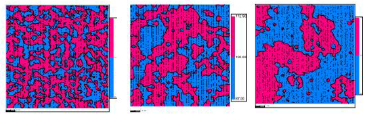
Figure 1: From left to right, the spatial structure increases but the coefficient of variation is the same.
- Geostatistical-based metrics: These are the indicators that are calculated after having constructed an experimental semi variogram and having fitted a theoretical variogram model to it (I invite you to reread previous posts on variography if it is no longer very clear). It is the parameters of this theoretical variogram model (range, sill, and nugget effect) that are mainly used to calculate indicators such as the Cambardella index, the MCD, or the Oi opportunity index (even if the latter is still a bit more complicated to calculate).
- Machine footprint-based metrics : For these indicators, we simulate the pass of a machine that will perform a given application, and we evaluate whether or not the machine will be able to take into account the spatial variability in the data. We will find in this category the technical opportunity index TOi, and its fuzzy declination, the FTOi, which uses the same concepts as the TOi, adding fuzzy logic components (uncertainty of the machine positioning at each moment, uncertainty on the data measurement…).
- Zoning-based metrics : Here we find indicators that will compare the interest of a given within-field zoning with a uniform management of the same plot. It is therefore necessary to have already established a zoning of the agronomic parameter of interest, i.e. to have already imagined a differentiated application on the plot. We find here the zoning opportunity indicator (ZOI) which simulates the pass of a machine on the zoned plot to evaluate if the machine is able to take into account the zoning delimited (by considering the size of the machine, its capacity to pass from treatment A to treatment B etc…). A second indicator that has not been mentioned in the article but may also be of interest is the so-called Variance Reduction (VR) indicator, which evaluates how much the variance is reduced in each of the delimited zones compared to the initial variance in the plot. However, this indicator does not take into account the fact that a machine can pass through the plot (with its constraints of size, latency, etc…). The VR index is presented in the article “Validating a Digital Soil Map with Corn Yield Data for Precision Agriculture Decision Support” published in the Agronomy Journal.
What to watch out for before using these indicators
Data diversity
Keep in mind that all the data sets collected are different from each other. This may sound silly to say, but the processing that will be done on the data must be completely thought out according to the nature and characteristics of the data and the way in which they were acquired; and this is quite the case when one wants to calculate an indicator of heterogeneity (we will come back to this in the next section).
The choice of a data acquisition method and vector is generally fully justified! This choice may be constrained by agronomic specificities (e.g. the trellised architecture of a vineyard), the cost of data acquisition, the time spent in the field, or the skills or expertise required to measure the agronomic parameter of interest as accurately as possible. Depending on these choices, the data will, for example, have a higher or lower spatial resolution (this is the density of observations), and the data may be regularly or irregularly distributed in space.
The data collected also have their own characteristics depending on the measurement support (soil, plant, etc.). For example, some data will be more or less self-correlated and structured in space [this is what we are trying to measure with an indicator of spatial variability]. Some datasets can be considered as spatially stationary, others not. As a reminder, the stationarity hypothesis is the fact that metrics such as the mean or variance are assumed to be stable over any considered space – we will recall here that this is one of the strong hypotheses for variogram modeling (I invite you to reread an old blog post on variography to refresh your memory).
In the article we wrote, we tested these four characteristics on simulated data sets to study their impact on heterogeneity indicators commonly used in the literature.
Characteristics of indicators of spatial variability
What we realize, without going into detail (I invite you to read the full article), is that the 4 criteria we have varied have an impact on the value of the indicators of spatial variability. So you can tell me that this is rather reassuring when it comes to the level of autocorrelation or spatial structure because it means that the indicators are able to discriminate data sets with different levels of spatial variability. And I will tell you that this is indeed the case even if all the indicators do not all have the same sensitivity to these different levels of spatial variability. This is not necessarily very serious as long as we know it after all!
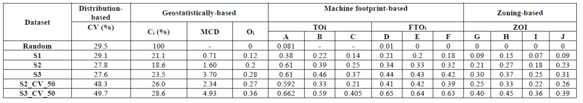
Figure 2. Sensitivity of indicators of spatial variability to autocorrelation in the data. Simulated data S1, S2 and S3 refer to weak, medium and strong spatial structure respectively. A to J stands for different footprint characteristics of the machinery
On the other hand, where we should start paying attention is when we vary the density of available observations, the regularity of the observations, or the hypothesis of stationarity of the studied phenomenon. And we realize that these impacts are far from negligible! In other words, using the same heterogeneity indicator to compare data sets with different characteristics can sometimes lead to conclusions that are very far from reality. For example, one realizes that :
- The lower the density of observations, the less geostatistical indicators can be calculated, and the more indicators such as TOi or ZOi give the false impression that the plot is very well structured (contrary to FTOi which manages the lack of data quite well).
- We can’t calculate geostatistical indicators on non-stationary data (we already knew that).
- Having data regularly or irregularly distributed in space does not have too much impact on geostatistical indicators and those based on a machine footprint.
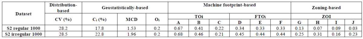
Figure 3. Sensitivity of spatial variability indicators to data regularity. A to J stands for different footprint characteristics of the machinery
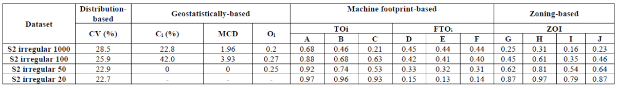
Figure 4. Sensitivity of spatial variability indicators to observation density. A to J stands for different footprint characteristics of the machinery
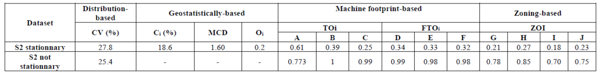
Figure 5. Sensitivity of spatial variability indicators to data stationarity. A to J stands for different footprint characteristics of the machinery
The characteristics of the data collected are one of the facets that it is important to take into account, but it is not the only one. From a very practical point of view, one must think of the user who wants to quantify the level of heterogeneity in his data. The choice of the indicator he will use will depend on aspects as concrete as the accessibility of these indicators on an existing tool or the ease of implementation of these indices. It is quite understandable that if an indicator is complex to calculate and, in addition to this, is not available on any GIS tool classically used, the user – despite all his good will – will not be able to consider it. Besides this, the level of expertise of the user in understanding the indicators must be taken into account. For example, some indicators are quite sensitive to the parameterization carried out by the user. In the same way as with the 4 criteria mainly tested, if the user does not clearly understand what he is doing, the conclusions will be wrong again. The most telling example concerns the fitting of a theoretical variogram model to the data. Depending on how the model is fitted, the geostatistical indicators can be very different!
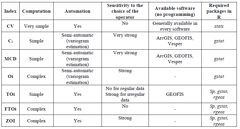
Figure 6. Calculation and accessibility of the different spatial variability indicators
Towards a joint and thoughtful use of indexes
At the end of this work on monitoring and benchmarking indicators of spatial variability, we realized that the choice of an indicator of spatial variability was far from obvious and that a decision tree was missing to guide us and find our way through this complexity. And this is what we produced in the last figure of this post. Choosing a suitable indicator of variability is certainly interesting in order not to make the data say anything, but it is also interesting to be able to compare experiments or results more easily with each other. Comparing different indicators of variability does not really make sense in itself as they each have their own sensitivity to the data. Perhaps this work will encourage stakeholders to standardize their measures of variability to get a clearer picture? Perhaps a more generic and standard indicator to measure this spatial variability is missing?
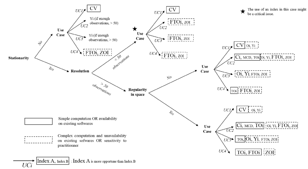
Figure 7. Decision tree to guide the choice of an indicator of spatial variability
Support Aspexit’s blog posts on TIPEEE
A small donation to continue to offer quality content and to always share and popularize knowledge =) ?