
Unless you have emerged from a period of cryogenics or have been locked in a bunker for several years, it is unlikely that you have never heard of a neural network. Having heard about it is one thing. Understanding what can be used is another. Knowing how it works is a whole different matter. If you look at what happens in the literature, in books or in some courses, you are very quickly buried under the equations (under the complicated terms and so on) without even really understanding what you are talking about. I wanted to make my humble contribution here to try to demystify and clarify certain concepts.
Neural networks, Deep learning and co.
In the family “I use catch-all words to shine in society without really understanding what it is”, I call “artificial intelligence”, “machine learning”, “deep learning” and “neural networks”. So, without really trying to redefine everything (there are some who will do it much better than me) but just to give a little background to this little world, we must understand that Deep Learning is a branch of Machine Learning, which is itself a branch of Artificial Intelligence. And when we talk about neural networks, we are referring to a type of algorithm for learning (the famous Learning). In agriculture, for example, a model can be taught how to predict wheat yields, how to identify a weed in a plot, or how to recognize a disease on a vine leaf. To learn this, we don’t have to use a neural network! Many different Machine Learning methods can be used such as decision trees, support vector machines (SVM), logistic regression, main component analysis and so on.
There are several different types of learning, the main ones being supervised learning, unsupervised learning, and reinforcement learning. We will come back to these terminologies at the end of the article, but what we hear most about neural networks is supervised learning. In simple terms, we talk about supervised learning because we will help our model to learn in the sense that we have input data for a model, and we know the outputs to which the model should arrive. If I use the example of wheat yield prediction, I have access to a number of model input data (soil type, climate data, agricultural practices, etc.) and I know the yield obtained with these input data, i.e. I know the model outputs. Using a supervised learning, I ask my model to learn how to find the yield from the input data I provide. And since the exact yield is known, the model can learn and improve itself. Again, what has just been described – supervised learning – can be developed with methods other than neural networks!
Architecture of neural networks
To stay consistent throughout the rest of the article, let’s stay on our example of yield prediction!
Let’s start with the simplest architecture of the neural network: a network with a single layer of a single neuron (Figure. 1). In this very simple example, we will use 3 input data:
- a_1 – the annual rainfall,
- latex]a_2[/latex] – the average annual temperature, and
- latex]a_3[/latex] – the soil type (each type of soil will be considered to have been labelled with a number).
These input data are used to feed a model composed of a neuron in order to produce a yield estimate (the small hat on the “y” is there to specify that it remains an estimate). To begin simply, our objective is to estimate whether the year’s yield will be “high” or “low”.
Forward propagation : How does the yield is estimated ?
To produce our yield estimate, the neuron here will perform a weighted sum of the available input data. To each input data, the neuron will associate a weight (the w_1,w_2, w_3[/latex]) and this is the weighted sum of these weights with the input data (\sum_{i=1}^{3} w_{i}a_{i}{i} = w_{1}a_{1} + w_{2}a_{2} + w_{3}a_{3}{3} ) which will be used to estimate a yield. These weights should be understood as an influence given to each input data. If, for example, rainfall is much more important than temperature in our yield prediction, the weight [latex]w_1 will be much greater than the weight w_2.
In our example of binary yield prediction, we can imagine that if the weighted sum of the inputs \sum_{i=1}^{3} w_{i}a_{i} is greater than a threshold, then the yield will be "high" (output 1) and if it is lower than the same threshold, then the yield will be "low" (output 0). We can consider that if our prediction led to a "high" output, it is actually that our neuron was activated (the weighted sum is higher than the threshold), while it remained asleep or deactivated (call it as you prefer) if our prediction led to a "low" output. See here a parallel with how our brain works with a number of neurons that may or may not activate to give a bunch of different reactions (the arrows between the inputs and the neuron can be seen as synapses).

Figure 1 : Architecture of a perceptron - Linear combination of inputs
So far, I hope everyone is still comfortable. In fact, a linear combination of inputs was simply used to predict low/high yield. Well, if neurons were only used for that, we wouldn't talk about it that much... The architecture that has been presented here (a layer of a neuron) is called a perceptron. It is the basic brick that will be used in neural networks.
Are you ready for the next step? Let's now add some notations:
If we use the idea of a threshold that we talked about to describe whether or not the neuron is activated, our little case study can be written simply with the following two conditions:
Si \sum_{i=1}^{3} w_{i}a_{i} > Seuil, alors Output 1: Yield "High"
Si \sum_{i=1}^{3} w_{i}a_{i} \le Seuil , alors Output 0: Yield "Low"
In reality, these two inequalities do not suit us very well... and to simplify our lives a little (and to simplify notations a lot later!), we will use a term "b" known as the perceptron bias. Our previous inequalities will now be written like this:
Si \sum_{i=1}^{3} w_{i}a_{i} +b > 0, alors Output 1: Yield "High"
Si \sum_{i=1}^{3} w_{i}a_{i} +b \le 0 , alors Output 0: Yield "Low"
This bias can be understood as the ease of activating a neuron. If the bias is very high, the neuron will be activated without any problem. On the other hand, if the bias is very negative, the neuron will not activate!
To further simplify the notations, we will call "z" our term to the left of the equation:
Si z > 0, alors Output 1: Yield "High"
Si z \le 0 , alors Output 0: Yield "Low"
Let's go back to our perceptron with these new notations (Figure 2). For the moment, what we have put in place is a model to predict a high/low yield from a linear combination of rainfall, temperature and soil type. The problem is that in most cases, it's still a little more complicated than that... We may want to predict a more accurate yield (with a numerical value or with many more classes than just high/low). This is a first problem because with the architecture we currently have, the model is only able to activate a neuron or not to activate it so we can't go much further than our binary classification (we may for example want a neuron that activates at 40%). And then, we can be relatively limited by the use of linear relationships between our input and output variables. In the agro-environmental world, we still very often face phenomena that we cannot model in a linear way. But then, how do we get out of all these constraints? With the activation function of course!

Figure 2. Architecture of a perceptron - New notations in place
The activation function is the function that will be applied to a neuron to decide whether or not it will be activated. It is a function that we will therefore apply to our entity z, and that we will note \phi (Figure 3).

Figure 3. Architecture of a perceptron - Activation of a neuron
And there are many activation functions, each with its own specificities. I'm just going to introduce three of them, but keep in mind that there are many more. The first one is the "step" activation function [Figure 4, left] and we can see that this function returns only two values over its entire interval: 0 or 1. It is simply the activation function that we have used so far in our case study!
To go a little deeper into neural activation, two other activation functions can also be used: the "sigmoid" function (which is noted instead \sigma and not \phi), which looks like an S [Figure 4, center] and the "ReLU" function (which is noted instead R and not \phi). Note that these two functions are non-linear! This makes it possible to overcome the limits of the linear combination we have seen previously. Concerning the "sigmoid" function, on its definition interval, we already realize that the function can return more values than just 0 or 1, which still leaves more flexibility on whether or not neurons are activated. The sigmoid function is very flat for very low or very high values of our variable "z". On the other hand, when "z" takes values between -2 and 2, the slope of the curve becomes very steep, which means that small changes in the value of "z" are able to have a relatively strong influence on the value of "z" and therefore on the activation or not of neurons.
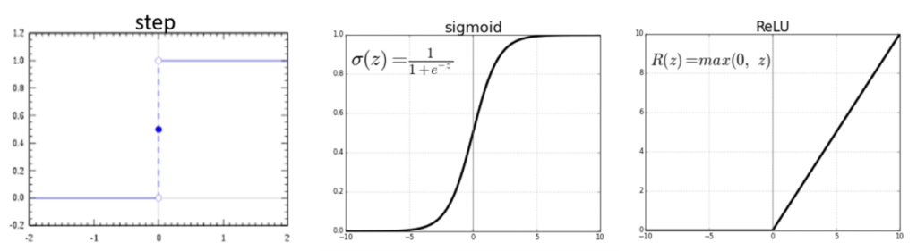
Figure 4. Exemples of three different activation layers
In practice, the "ReLu" function is used more than the "sigmoid" function.
What happens in this paragraph is not fundamental to understanding the remaining, it's just for curious people (and you can come back to it at the end of the article, it will certainly be clearer): For those who are interested, the "ReLu" function is more used than the "sigmoid" function because the "sigmoid" function is subject to the phenomenon called the "vanishing descent problem". We will see it again a little later but to evaluate the weights,w_1,w_2,w_3 of our neural architecture, we will have to go through a backpropagation step. In this step, the objective will be to minimize a cost function (which is none other than the error of our model). And to minimize this function, it will be necessary to calculate error gradients in relation to these weights (the famous gradient descent), gradients that will become smaller and smaller as we have many layers and as we try to go back to the neurons of the first layers. Because of the flat tails of the sigmoid function, one can find oneself "stuck" at these tails, with neurons that have difficulty to learn, especially the neurons of the first layers. And these neurons are particularly important because they are the ones who will extract the big patches and trends in our data (and so we need them to learn well!).
To get back to the "ReLU" function, we observe a flat curve for values of "z" less than 0 and a linear function for values of "z" greater than 0. Be careful, it does not make it a linear function over its entire interval, it remains a non-linear function!
Another small point for the curious: We are therefore partly free of the phenomenon of "vanishing descent problem" here unlike the "sigmoid" function. However, there are still some (less important) problems, in particular the fact that neurons for which the values of "z" are less than 0 are generally considered dead since they cannot be reactivated (the slope is completely flat so the calculated gradients will not change). Alternatives exist, such as the "Leaky ReLU" which, instead of having a "flat" curve for values of "z" lower than 0, has a linear curve with a slight slope.
Well, once we have all our architecture (the input data, our 1 neuron layer, and our activation function), we will try to predict our yield. Small problem and not the least: How to fix the weights w_1,w_2,w_3? Basically the question is, how does our model learn? It's backpropagation
Backpropagation : How does the model learn?
If we are still on the same page, we want to use our three input data (rainfall, temperature, soil type) to predict whether the year's yield will be "low" or "high". To build and evaluate a prediction model, what is traditionally done is to separate its data set into a training set, and a validation set. The model "learns" with the training set, then the model is validated on the validation set. We will therefore focus here on a learning set, i.e. a set for which the inputs and outputs are known. We therefore have a set of training data that we can see as a table with, in rows the different study sites, and in columns, the values of rainfall, temperature, soil type, and yield obtained (low or high).
As shown in Figure 3 in our simplified case study, the yield predicted with our model is written \phi(z). Our model can be considered good if it is able to find the right output value "y" (true yield) associated with the corresponding input data. We can therefore construct a simple error function (also called model cost) C_{x} for each of the study sites x.
C_{x} = [\phi(z(x)) -y(x)]^2
On this cost function, sites for which the yield was poorly predicted are penalized (with the square). The objective, not surprisingly, is to try to minimize this cost function, which means that we are trying to minimize prediction errors at the study sites. From this cost function per study site, a cost function can be constructed for the entire model, which is the average of the costs associated with each study site
C = \frac{1}{n} \sum C_{x}
Withn the number of study sites
It must be understood that this cost function simply tells the model whether or not it has done its prediction work properly. But it doesn't tell him how to improve... In fact, what we're really trying to do is to find the best input weights of the model (our w_1,w_2,w_3 and do not forget the neuron bias b !) to make the model predict the best possible. At the beginning, the weights are set randomly (we will come back to this later) but as the model learns, the model must be helped to understand in which direction it must change its weights and bias to improve the predictions. And for that, what better way to do it than to use derivatives! Well yes, what we want to calculate is the derivative of the cost function with respect to w_1 to know how to change w_1 to minimize the error or cost of the model, and the same for w_2, w_3 and b.
Let's go, at least for w_1 (and it will be the same for w_2, w_3 and almost the same for b) ! A little bit of math is great ! We will therefore calculate the derivative of our cost function with respect to w_1, which we will note \frac {\partial C_{x}}{\partial w_{1}}. We will be able to calculate this derivative as follows:
\frac {\partial C_{x}}{\partial w_{1}} = \frac {\partial z(x)}{\partial w_{1}} \times \frac {\partial C_{x}}{\partial z(x)}
We recall the formulas of z and C_{x} that we will use :
z(x)=w_{1}a_{1}(x) + w_{2}a_{2}(x) + w_{3}a_{3}(x) + b(x)
C_{x} = [\phi(z(x)) -y(x)]^2
We will calculate a variation of the cost function with respect to w_1 for each study site and then we will apply the average of all these variations to w_1 as we will see later. Now, let's derive the formulas of the previous z(x) and C_{x} in order to calculate \frac {\partial z(x)}{\partial w_{1}} and \frac {\partial C_{x}}{\partial z(x)}.
\frac {\partial z(x)}{\partial w_{1}} = a_{1}(x)
\frac {\partial C_{x}}{\partial z(x)} = 2 \times [\phi(z(x)) -y(x)] \times \phi'(z(x))
Thanks to these formulas, we know how to vary the weight w_1 to improve our model! I would remind you that the variation in the cost function with respect to w_1 was calculated for a study site x and that it is the average variation on all study sites that interests us to know how to vary w_1
\frac {\partial C}{\partial w_{1}} = \frac {1}{n} \sum_{x} \frac {\partial C_{x}}{\partial w_{1}}
We then vary w_1 using the following formula:
w_{1} = w_{1} - \eta \times \frac {\partial C}{\partial w_{1}}
With \eta the learning rate (or learning rate in English) that the user sets as the hyperparameter of the model (we will come back to this notion of hyperparameter). You may sometimes see the learning rate also noted \alpha. We can see the term \eta as the speed with which weights and biases will converge to their optimal value, and therefore the cost function will converge to its minimum value. But let's just take a value of \eta super high then!?! No....... The problem is that if you use a value of \eta too large, the algorithm may diverge instead of converging! We can say that the weights and biases try to converge so quickly that they miss their optimal value and will be completely lost... If we take a low \eta value, the algorithm will converge too slowly, which is not necessarily problematical, unless the cost function gets stuck in a local minimum, and therefore does not reach its global minimum, i. e. its optimum. Therefore, you should choose relatively carefully the value of \eta. Values can be found in the literature or on existing models that do not work too badly. It is then up to the user to rework his or her settings. I didn't clearly mention what we've seen so far, but in fact, we just talked about the gradient descent ("gradient descent") which is often scary! The gradient descent is actually nothing more than the term " - \eta \times \frac {\partial C}{\partial w_{1}} ". There is a negative sign because we are looking for the direction to decrease the cost function and we are talking about a gradient because of the derivative of the cost function with respect to w_1. The hyperparameter \eta allows to add a notion of proportionality.
Note: you can see \frac {\partial C}{\partial w_{1}} noted in a simpler way dw_{1} :
w_{1} = w_{1} - \eta \times dw_{1}
It is then sufficient to do the same thing again to update the values of w_2, w_3 and b (this is not done here but it is the same principle).
If we quickly summarize what is happening with neural networks, in fact:
- We initialize the weights of the network (we will come back to them later but we must start from existing weights at the beginning before changing them)
- For each study site x
- We make a prediction (it's the forward propagation)
- We calculate the cost of the prediction associated with the site x
- We calculate the derivative of the cost function with respect to the weights and biases of the model (it is the back propagation)
- The results are averaged over the entire dataset and the network weights/biais are updated
Extension to the multi-layers neurons
The previous example is relatively simple, we will not hide it, but it has made it possible (I hope) to clarify a certain number of concepts. In the architecture of the perceptron we have seen, there is indeed only one layer composed of a single neuron. For the complex tasks that everyone is likely to have to perform, this architecture is not sufficient. It will indeed be necessary to add layers and neurons per layer but no worries, all the concepts we have seen remain relevant; we will only add a few notations so that all our previous equations can be extended to the case of multilayer or "deep" neural networks. Depth is what we mean when we add layers to the neural network, to allow the model to discover and learn more and more complex relationships. The perceptron is a simple network since there is not only one layer (we can talk about "shallow" learning to differentiate it from deep" learning). Let's see below a more complicated architecture:
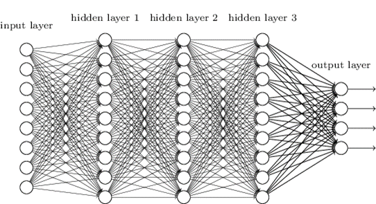
Figure 5. Architecture of a multi-layer perceptron
We can see here a layer with input data (input layer), three layers that are said to be hidden because they link the inputs and outputs (hidden layers 1, 2 and 3), and the output layer. In this example, each hidden layer is composed of as many neurons but this is not necessarily the case! We also see several output layers, which can appear counter-intuitive at first. But imagine if you wanted to predict four yield classes (Very Low, Low, High, Very High), then you will need four outputs with the probability of belonging to each class for each.
With this new architecture, you can start to feel that we will have to manipulate a lot of input data, a lot of weight (each line on the figure represents a weight) and a lot of bias (one per neuron). It is therefore necessary to clarify some notations! In the perceptron architecture, we have called a_1,a_2,a_3 the input data of our model,w_1, w_2, w_3[/latex] the weights associated with the three input data used, b the neuron bias of our model and z the sum of the bias and the weighted sum of the inputs \sum_{i=1}^{3} w_{i}a_{i}+b. Nothing complicated but now look at the new notations:
- w^{l}_{jk} is the weight of the connection between the neuron k of the layer l-1 and the neuron j of the layer l.
- b^{l}_{j} is the bias of the neuron j of the layer l
- a^{l}_{j} is the activation of the neuron j of the layer l1\phi(z)[/latex]].
The input data layer is layer 0 and in general it is not counted when counting the number of total layers in the neural architecture. L is the number of layers in the neural network so also the number of the last layer (again we don't count the first one). With a figure, it will be even clearer (a little smaller than the previous one to see something).
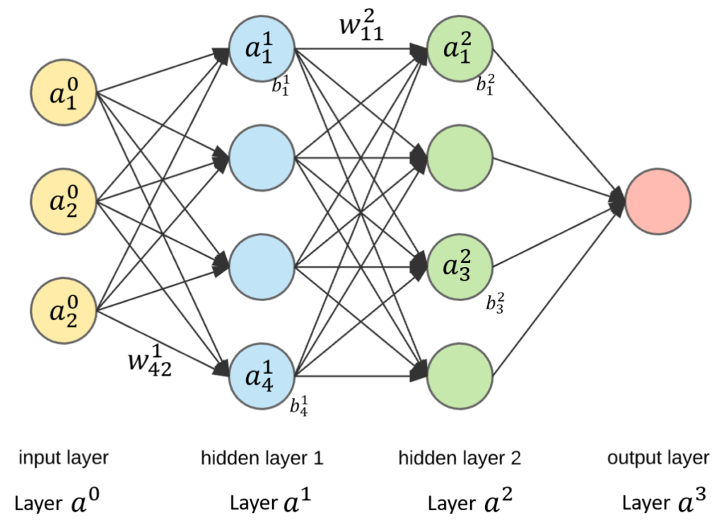
Figure 6. Architecture of multi-layer perceptrons with the new notations. There are here L = 3 layers
With these new notations, we realize that we will be able to easily link the activation of a neuron on a layer with the activation of a neuron bound to it on a previous layer:
a^{l}_{j} = \phi (\sum_{k} w^{l}_{jk}a^{l-1}_{j}+b^{l}_{j})
We can see the parallel with our previous notations:
\phi(z) = \phi (\sum_{i=1}^{3} w_{i}a_{i} +b)
And if, to further simplify the notations, the previous equation is written in a matrix form
a^{l} = \phi (w^{l}a^{l-1}+b^{l}) = \phi(z^{l})
And so, we have generalized our architecture to a multi-layer neural network! We're not going to stop there! These notations can be used to also extend the cost function and backpropagation to a multi-layer network:
C_{x} = [a^{L}(x) -y(x)]^2
Here, it is the index L that is used since it is the index of the last layer of the neural network, i.e. the output layer and it is this one that must be compared to the true yield value y(x) corresponding to the study site x. Similarly, the cost function for the entire model (and not just a study site) is written:
C = \frac{1}{n} \sum C_{x}
Withn the number of study sites
For backpropagation, we again try to evaluate the derivative of the cost function in relation to all the weights fixed in the model (and also in relation to neural biases, we don't forget them!):
\frac {\partial C_{x}}{\partial w^{l}} = \frac {\partial z^{l}(x)}{\partial w^{l}} \times \frac {\partial a^{l}}{\partial z^{l}(x)} \times \frac {\partial C_{x}}{\partial a^{l}}
\frac {\partial C_{x}}{\partial b^{l}} = \frac {\partial z^{l}(x)}{\partial b^{l}} \times \frac {\partial a^{l}}{\partial z^{l}(x)} \times \frac {\partial C_{x}}{\partial a^{l}}
Note that here, compared to the first simple architecture we used, we added the activation terms a^{l}. Then follows the same derivation work as before (with the updated formulas of course) that I will not detail here. These calculations allow you once again to find out how to vary the weights of your model to improve it. Variations are averaged over all study sites:
\frac {\partial C}{\partial w^{l}} = \frac {1}{n} \sum_{x} \frac {\partial C_{x}}{\partial w^{l}}
\frac {\partial C}{\partial b^{l}} = \frac {1}{n} \sum_{x} \frac {\partial C_{x}}{\partial b^{l}}
We then update the weights and biases:
w^{l} = w^{l} - \eta \times \frac {\partial C}{\partial w^{l}}
b^{l} = b^{l} - \eta \times \frac {\partial C}{\partial b^{l}}
Some references to look at!
- A set of some videos with very nice illustrations: https://www.youtube.com/channel/UCYO_jab_esuFRV4b17AJtAw
- A very detailed online book on neural networks: http://neuralnetworksanddeeplearning.com/
- Some websites with relevant animations/information:
Support Aspexit's blog posts on TIPEEE
A small donation to continue to offer quality content and to always share and popularize knowledge =) ?
1 thought on “Neural network – Let’s try to demystify all this a little bit (1) – Neural architecture”