
A short break from the classic files I write to return to my first love of spatialized data processing!
This “small” dossier allows me to share and valorize the work done with a wine château during several vintages in a row.
This chateau has the time and the means to collect high resolution data, but also the motivation to understand and engage in a reflection work around this data.
In this work, I propose a methodology to synthesize the information contained in historical data (7 years and more) of intra-parcel vegetation maps on large domains. I will bring you here some methodological and theoretical elements, but I will try to show you that in operational contexts, it is necessary to accept to make a certain number of sacrifices, whether it is in terms of quality of collected data or of information processing chain. I am obviously not saying that we can accept to work like pigs – we must strive for the best – but it is necessary to adapt to field conditions. The reality is often less rosy than the theory.
Anyway, back to our methodology. The approach presented here consists of providing two different indicators:
- an indicator of spatial heterogeneity of vegetation, or in other words: “is the plot homogeneous or heterogeneous?”
- an indicator of temporal instability of vegetation, i.e. “are the vegetation structures within the plots stable or not over time?”
These indicators, used in relative terms, allow us to prioritize the plots in terms of spatial variability over time in order to prioritize modulated interventions on certain plots rather than others or to (re)-organize the allocation of the plots in the domain. These indicators are also a way to evaluate the interest of comparing variations in vegetation with cultivation itineraries implemented in the plots. Understand here that if the spatial structures and patterns of vegetation evolve a lot in time, there is still a good chance that this is due to the itineraries chosen on the plots concerned.
The methodology, used here in the context of vegetation data in viticulture, is redeployable in other sectors and for other types of agronomic data where long histories are available.
The bibliography is short and rather self-centered, but you will find many other references in it that I hope will be useful to you. The purpose of this file is essentially to share an operational feedback.
[mailpoet_form id=”1″]
Soutenez Agriculture et numérique – Blog Aspexit sur Tipeee
Why did we do this work?
It is not easy to use high-resolution data acquired on a given plot at a given date. Nevertheless, this data remains accessible to the human eye if we make the effort to present it at least in a cartographic form. This data can be difficult to understand if it is not transformed into agronomic information, but the number of dimensions around this data (a year, a plot, a variable) remains relatively low.
When one starts to increase the number of plots studied, and this over several years, it becomes very difficult to abstract from this complexity, to identify trends, and to step back from what is really happening on the farm. The dimensions around this data are too large for our brains to be able to synthesize on their own and we can then be biased in their interpretation.
And the sources of bias are terribly numerous… Colors of the data display, size and shape of the plots, number of years of analysis, personal experience in the field; the list goes on. These biases are already present when looking at within-field mapping. So when we look at historical maps on large domains, I let you imagine what happens next. A quick digression around the color bias of maps. I would be tempted to ask several different operators to delineate vegetation zones on fields using maps with different color gradients. Exactly the same data processing but just with the gradient colors changing (from green to red and blue to green for example). While I expect differences between operators, I am also confident that the same operator would be able to slice the same plot differently if the color gradients are changing.
The deployment of digital tools for several years now favors the acquisition of multi-dimensional data (several variables, several plots, several years) – recurrent passages several times in the season and/or over several seasons to follow the evolution of agro-pedo-climatic parameters. In the precision agriculture community, several authors have already attempted to synthesize this complex information, but often on one or the other of these dimensions. One can think, for example, of some work on modulation opportunity indices (Leroux and Tisseyre, 2018a) to try to describe, in an indicator, whether a plot has a sufficient magnitude of variation and spatial structure for it to be relevant to imagine a modulated application there. The issue here is spatial and these indicators are not necessarily comparable from one plot to another. As far as the synthesis of temporal information is concerned, the first thing that comes to mind is perhaps the first work on historical yield maps (those of Simon Blackmore, for example) to identify, within the same plot, stable and unstable yield zones over time. The issue here is a temporal one, where we generally work within a single plot and do not seek to compare plots between them.
Inspired by all these works, we tried here to work both in the spatial domain and in the temporal domain to compare plots for which we had historical vegetation maps.
Material and methods
Data sites
We worked on 2 different wine growing sites in the Bordeaux region:
Site 1: About 150 plots, a little more than a hundred hectares, 2 majority grape varieties (Semillon, Sauvignon Blanc),
Site 2: A little more than 200 plots, nearly 250 hectares, 3 main grape varieties (Cabernet Sauvignon, Merlot, Petit Verdot)
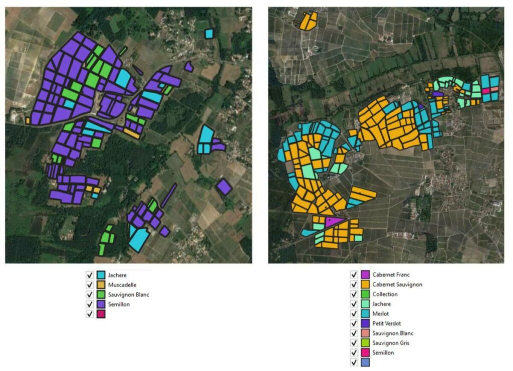
Figure 1. The work sites (1 on the left, and 2 on the right)
On these 2 sites, the domain team had at its disposal a certain number of historical vegetation maps – over 7 years for site 1, and over 8 years for site 2. Not bad already, you might say, but it’s starting to look pretty good! Well then, green light ! Let’s calculate these heterogeneity indicators and call it a day? Let me come back to the fact that these data are not completely homogeneous. Yikes! The operational context of the work is part of the reason why the vegetation data are different from year to year. The suppliers of vegetation maps have changed over time (so the same data acquisition and pre-processing methodology has changed as well), the sensors and technologies may have also evolved over time, and the thinking of the vineyard has necessarily matured as well. Tables 1 and 2 give you some initial information on the data available and on the data harmonization that we have undertaken.
Table 1. Characteristics of the vegetation data available for site 1. The data are globally acquired on the same period each year (July)
| Year | Data | Provider | Harmonisation process or comment |
| 2011 | NDVI (4 GreenSeeker on straddle carrier) – no white reflector | A | Individualized data on the row for each of the 4 sensors available |
| 2012 to 2016 | NDVI (3 GreenSeekers on the tractor) -with white reflector | A | The data from the 3 sensors are directly averaged during the acquisition (there is no individual data from each sensor that can be recovered). The very low values of vegetation (missing feet or other) are thus directly averaged and not separable from the rest of the data (if one had wanted to separate them for example). Sensor bugs and sensor changes during the period |
| 2017 to 2019 | NDVI (3 GreenSeekers on the tractor) -with white reflector | A | Individualized data for each of the 3 sensors available |
| 2020 | EVI on the row (plane flight) | C | Not used in this work |
Table 2. Characteristics of available vegetation data for site 2. The data are globally acquired on the same period each year (July)
| Year | Data | Provider | Harmonisation process or comment |
| 2016 | Reflectance without distinction of the inter-row (plane flight) | B | No NDVI data. Information on 4 bands with reflectance values (0 to 255). Raster format. These are not the raw data, the data had already been smoothed |
| 2017 | NDVI on the row (airplane flight) | B | |
| 2018 | NDVI on the row (airplane flight) | B | Pre-classified NDVI data, these are not raw data (which are no longer accessible). The data is in regular gridded form (it is not point data like the rest of the data). It seems that a raster has been classified and then vectorized brutally without pre/post-processing |
| 2019 | NDVI on the row (airplane flight) | B | |
| 2020 | EVI on the row (airplane flight) | C | |
| 2021 | EVI on the row (airplane flight) | C | Long treatment of the supplier because of a very rainy year which made the weed very visible |
| 2022 | EVI on the row (airplane flight) | C | 2 passes, one during the summer and one just before harvest (only the summer pass was used) |
We tried to harmonize the data as much as possible in order to obtain point data on vegetation on all the plots, with consistent attribute tables. We have accepted that the vegetation indicators are not the same from one year to the next, and we have made sure that we work in relative terms from one year to the next in order to compensate for these effects (we will discuss this further below).
And since the objective is to give you feedback, I would like to share with you some of the joys experienced during the work. Joys for which you will need a punching bag, a soundproof room, advanced meditation exercises, and potentially calling mom if you are really at the end of your life:
- the data provided are not always in the same reference coordinate system (https://www.aspexit.com/les-systemes-de-coordonnees-de-reference/). And that’s when you are lucky and a reference coordinate system is present…
- the attribute tables of the layers are not always structured the same
- the parcels have topology and/or attribute defects: some parcels overlap, some have holes that we don’t really know how they got there, others are split into several disjointed parcels but have the same identifier
- some data are missing and you end up realizing that some parcels have not been processed because the data were not present in the initial file
- the parcel system has evolved over time, but you learn this at your expense a little late
- the metadata of the layers are not filled in and we don’t really know when the data were acquired or digitized
- the cultivation itineraries on the plots, especially for the first years of vegetation, are not always well known and followed
- ….
I am obviously exaggerating a bit here, as the time spent cleaning and preparing the data is often underestimated. Nevertheless, I would like to underline the great efforts and the will of these two wineries to already make a state of the art of the available data and then to centralize the existing data in order to be able to exploit such a data history. These first works serve to wipe the slate clean and to share feedbacks from which the following ones can be largely inspired.
Zoning vegetation maps
The harmonized vegetation data were zoned (clipped), year by year, using a growth and then zone merging algorithm inspired by the field of image segmentation, but applied to point data (Leroux et al., 2017). Figure 2 presents this approach in a pictorial form. In more accessible terms, let’s say it’s like letting oil spots spread over the plots and gradually form larger and larger areas until the entire plot is covered in oil. The initial number and position of oil spots is chosen according to the variability observed in the plot.
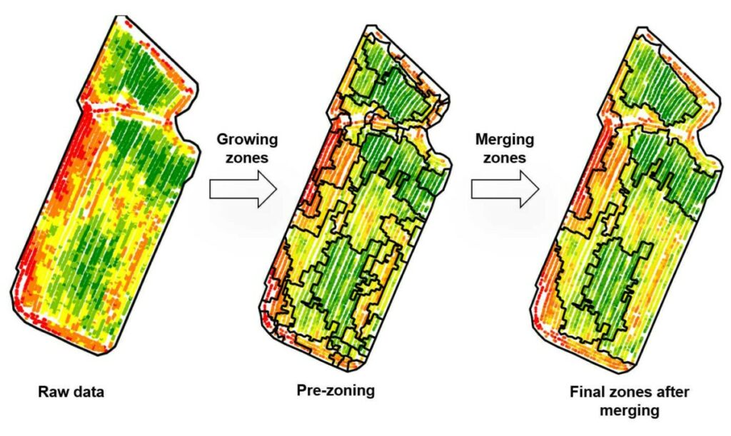
Figure 2: Methodology for automatically zoning (cutting) a plot.
Although multi-annual zoning would have been possible, i.e. proposing an aggregative zoning of several years at once (this was proposed during my thesis – Leroux et al., 2018b), it was decided here to perform an annual zoning because the vegetation data sources were, initially, relatively different between years (see the section “Sites and Datasets”). The comparison of zonings between years is done in a second step (see next section).
For each year and each plot, the final number of zones (Figure 2) is defined automatically by the algorithm based on a stopping criterion during zone merging (Leroux et al., 2017). Thus, the number of zones is potentially different between each plot in the same year and/or between each year in the same plot.
To simplify the zonings at the whole plot scale, the median values of each vegetation zone were classified, year by year, across all grape varieties, into 6 different classes using an equal interval classification. Neighboring vegetation zones with the same vegetation class value were thus merged, the process resulting in a coarser zoning than that obtained at the end of the automatic zoning algorithm (Figure 3).
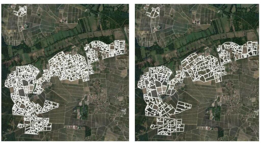
Figure 3. 2020 vegetation zoning for site 2. Left, after growth and zone merging. Right, after further classification into 6 vegetation classes
It is this zoning, constructed from the harmonized vegetation data, and the zoning algorithm of Leroux et al., (2017) that will be used in the remainder of this study.
Comparing zonings in time
From an operational point of view, it is interesting to distinguish :
- Homogeneous plots and heterogeneous plots, so as to be able to prioritize the plots that could be the site of modulated application or reorganization, and
- among the heterogeneous plots, those whose vegetation patterns are stable over time, i.e. those for which it is possible to reason over the long term, and, on the contrary, those whose vegetation patterns vary over time, i.e. those for which management will be more reasonable over the short term
Two indicators have been provided for this purpose, which are detailed below. The calculation of these indicators is also shown in Figure 4.
Evaluation of the heterogeneity of the plots
For each plot and year, the plot zoning was used to calculate a zone variance reduction (VR) index (see equation below), which is an indicator of the ability of the zoning to represent subjacent spatial variability in the vegetation data (Bobryk et al., 2016). This indicator ranges from 0 to 1. Close to 0, it basically tells you that your zoning is not doing much good because the variability in each of the zones is broadly the same as if you had done nothing. For example, if you had a plot where the northern half was very vigorous, the southern half was very weak, and the zoning algorithm suggested an east-west split. So, you can always tell me that it’s the zoning algorithm that’s potentially bad – and you’d be right – but we’re going to assume that the algorithm isn’t talking nonsense and that a post-zoning visual check ensures that the zoning is consistent with the data.
If the variance reduction index is close to 1, then the variability in each zone has largely decreased compared to the total variability in the plot. In reality, the index is never really 1 because that would mean that all the data are exactly the same in each zone or that each zone contains only one point data.

Translation : Numerator [Sum of zones variances (weighted by the area of the zone)] and Denominator [the total variance of the field]
For the rest of the record, I note here RV_i,j,k the variance reduction index for plot i, using vegetation data from year j, and zoning from year k. You may be surprised to see that I use two different letters to refer to the years, but this is because you will see that I am proposing to plot zonings from a year j on vegetation data from a different year k, especially for the 2nd proposed indicator (Figure 4). Patience patience…
The first heterogeneity indicator (the multi-year heterogeneity of a plot, which we will note Het_i), i.e. the one that answers the question: “is the plot homogeneous or heterogeneous?”, is defined as the average of the variance reduction indices over all the years for plot i, when the year of the zoning is identical to that of the vegetation data:
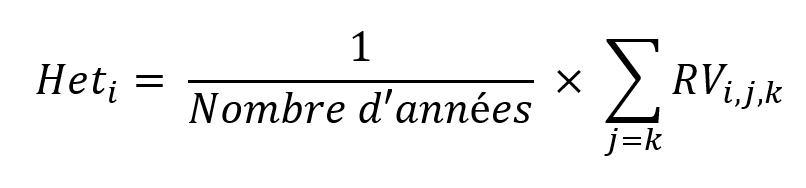
Translation : Denominator (Number of years)
Assessment of the instability of heterogeneity over time
It is considered here that a vegetation pattern is stable over time if each zoning in any year can be used to represent the spatial variability of another year in a consistent way. If two vegetation patterns are very different between a year j1 and j2, i.e. the spatial heterogeneity is not stable over time, the vegetation zoning on year j1 will represent the spatial variability on year j2 very poorly. The underlying idea here is to map, for each plot, the set of available zonings onto each of the initial vegetation data (Figure 4): a sort of cross-tabulation that makes it possible to compare two by two a zoning of a given year to the vegetation values of a different year. It is assumed that the best zoning of the data of year j is the one realized using these data (Figure 4). The difference between this optimal value and the variance reduction values obtained with zonings from different years is therefore compared.
The lower the instability indicator, the more stable a plot will be over time.
The second indicator of heterogeneity (the temporal stability of the vegetation pattern on a plot, which we will note Instab_i), i.e. the one that answers the question: “are the vegetation patterns consistent or not over time? “is defined as the average of the absolute differences between the variance reduction index calculated by plotting zonings of a year k on vegetation data of a different year j (j different from k), and the one calculated by plotting zonings of a year k on vegetation data of a same year j (j equal to k)
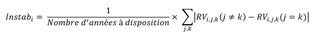
Translation : Denominator (Number of years at disposal)
Figure 4 below shows schematically how the heterogeneity and instability indicators are calculated.
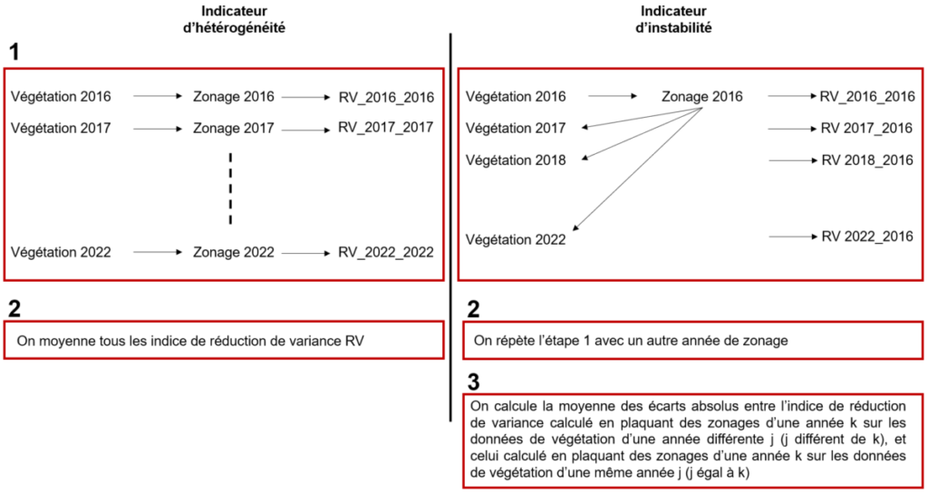
Figure 4: Steps for calculating heterogeneity and instability indicators.
Translation.
- Left (Heterogeneity Indicator). 2. Averaging all the reduction variance indexes RV
- Right (Instability Indicator). 2 Repeating step 1 with another zoning year. 3. Calculating the average of the absolute differences between the variance reduction index calculated by plotting zonings of a year k on vegetation data of a different year j (j different from k), and the one calculated by plotting zonings of a year k on vegetation data of a same year j (j equal to k)
Mapping indicators of vegetation heterogeneity and instability
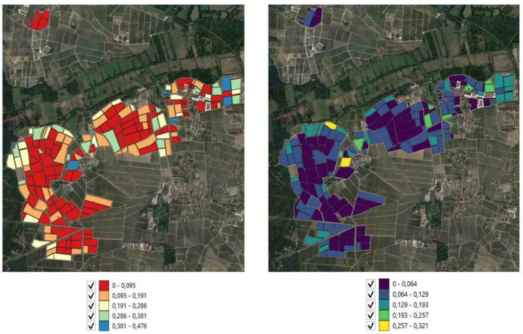
This is the result of the calculation of these two indicators on site 2 (Figure 5). I remind you here that these indicators synthesize information contained in large vegetation histories and that their main interest lies in their capacity to take a step back on the state of the vegetation on the domain.
Figure 5: Mapping of vegetation heterogeneity (left) and heterogeneity instability (right) indicators
These indicators are to be used relatively. They allow us to rank the plots in relation to each other but not to set thresholds for heterogeneity and/or temporal instability of vegetation. These thresholds, if they must be set, will be done by the vineyard managers using their expertise of the domain and their own representation of what is a sufficient level of heterogeneity. The thresholds can then potentially be reapplied under other operational conditions.
The explanation of the vegetation condition can be done at several levels:
- At the level of the entire plot (we could talk about a global scale): we will try to explain what we see in terms of global heterogeneity or global vegetation level by the vintage
- At the plot level: if the location of the vegetation heterogeneity changes on the plot, we will try to understand why with agronomic orientations (soil, useful reserve…) but also logistic ones (plots with broken drains, plots recently pulled out…)
- At the level of the area: if the areas are unstable over time, it would certainly be interesting to look for an explanation in the cultivation itineraries implemented (fertilization, grassing). In this first case, we would prefer short-term management of modulation or perhaps not to consider modulation at all because the risk of making mistakes is too great. If, on the other hand, the vegetation zones are stable over time, there is little point in comparing them with the crop itinerary. In this second case, it may be more interesting to work on the intra-plot level and to implement modulation practices because it will be possible to reason on a relatively long-term basis.
The zonings that are presented in this file are purely statistical. They do not really integrate professional expertise and are based solely on the harmonized vegetation data available. Work has been undertaken to integrate the professional and historical expertise of the domain’s staff into these zoning studies, including
- Manual re-refining of the zonings in the field after visiting the plots. This re-refinement is based on the experience and the representation that the estate staff has of its plots. It may be criticized that this representation is certainly broader than the vegetation alone and that it actually integrates several dimensions. But is this really so serious?
- The expert classification of vegetation zones in terms of visual appreciation in the field (Figure 6). It should be understood here that field operators were asked to rate a level of vigor from 1 to 3 in each drawn area, so that they could compare the vegetation data values in each area to the expert vegetation classes set by the field staff (the proposed classification was initially from 1 to 5, but this overly precise classification was not discriminating enough). The idea was to see if the vegetation data in each class were very well discriminated or overlapped. This analysis would then allow us to set a vegetation threshold for each of the classes (and thus to transform statistical vegetation classes into expert vegetation classes on the domain), and to reproject this threshold over different years (paying attention to the harmonization of thresholds since vegetation levels are significantly different from one year to another).
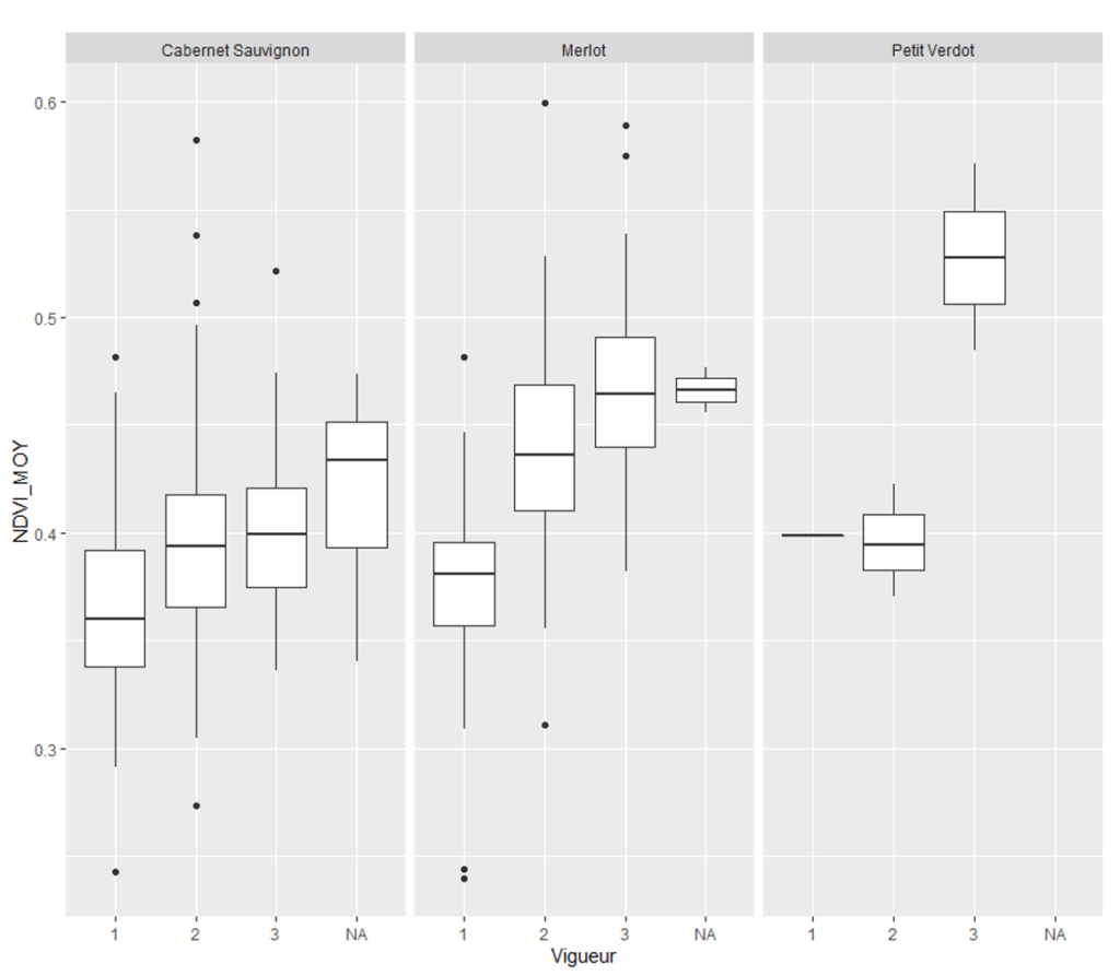
Figure 6. Match between expert vegetation classes (1, 2 and 3) and vegetation data (see Table 1 and 2) for the 3 majority grape varieties of site 2.
On the proposed methodology, far from being perfect, we can also identify some initial limitations:
- The variance reduction index is necessarily somewhat dependent on the number of zones in each plot. However, the relationship is not necessarily linear. Since the number of zones is not identical in each of the plots, there is necessarily still some bias
- We have given the same weight or influence to each of the available years. This is a choice we made, but we could also have given more influence to some years rather than others (the most recent ones for example).
- The zoning instability indicator looks at the shape of the zones, i.e. whether the zones remain more or less the same over time. It should be kept in mind that this indicator does not give any information about whether the vegetation in these zones can vary strongly. For example, one can imagine flip-flop effects with areas of high vegetation one year becoming areas of low vegetation the next, for example due to the effect of intense rainfall on a particular soil zone.
- Not surprisingly, the results presented here depend on the set of data processing methods applied, particularly the zoning and classification of the initial vigor data into 6 equally spaced classes.
The work with the vineyard also gave rise to the analysis of data complementary to the vegetation, in particular on the soil via conductivity data (for site 1) and on the climate with fairly rough representations of the different climatic years (proposed by the vineyard managers). The challenge is always to try to explain the observed variability of vegetation. The work on climate was not conclusive because it was relatively superficial. The 2017 frost potentially reshuffled the vegetation maps. The very rainy year of 2018 potentially deepened the levels of heterogeneity. The different data acquisitions (e.g. the 3 different periods for site 1) may have masked some vegetation variations. Let us also add that most of the key phenological periods of the vineyard take place after the data acquisition period.
In conclusion
Digital tools have the advantage of being able to objectively measure certain phenotypic parameters of the vegetation (NDVI, EVI…) with the limits that we know (correlation rather than causality, difficulty in linking to a real physiological state of the plant, use of these indices for decision making). But their use in an operational context is still largely a matter for specialists, and there are many technical and logistical constraints (change of service provider, data analysis changing over time, etc.).
The work of cleaning and formatting the data is a part-time job which is already very useful in itself in an operational context since it already allows us to start on a good basis. The work has allowed the staff of the domain to have harmonized and well recontextualized vegetation data.
In view of the recurrent exchanges with the staff of the domain, it appears necessary that new skills, especially in geomatics and spatial data manipulation, be internalized in these operational structures. These skills are important to understand the issues and limitations of data acquisition, to have control over the data acquisition and/or processing processes, and above all to be able to react when a provider changes or processing needs to be updated.
Spatio-temporal historical data – such as the vegetation data we have seen here – must be simplified if they are ever to be used in the field. Otherwise, we run the risk of being satisfied with collecting high-resolution data that will remain neatly stored in a drawer.
Bibliography
Bobryk et al., (2016). Validating a Digital Soil Map with Corn Yield Data for Precision Agriculture Decision Support. Agronomy Journal : https://acsess.onlinelibrary.wiley.com/doi/full/10.2134/agronj2015.0381
Leroux, C., Jones, H., Clenet, A., & Tisseyre, B. (2017). A new approach for zoning irregularly-spaced, within-field data. Computers and Electronics in Agriculture, 141 (C), 196-206. DOI: https://doi.org/10.1016/j.compag.2017.07.025
Leroux, C., & Tisseyre, B. (2018a). How to measure and report within-field variability – A review of common indicators and their sensitivity. Precision Agriculture. https://doi.org/10.1007/s11119-018-9598-x
Leroux, C., Jones, H., Taylor, J, Clenet, A., & Tisseyre, B. (2018b). A zone-based approach for processing and interpreting variability in multitemporal yield data sets. Computers and Electronics in Agriculture, 148, 299-308. https://doi.org/10.1016/j.compag.2018.03.029
Soutenez Agriculture et numérique – Blog Aspexit sur Tipeee