The complex architecture that we have detailed in detail in the previous sections is a multi-layer perceptron (MLP). This is the classic architecture of the neural network. Nevertheless, depending on the type of data used to input neural models (images, voice signal, etc.), more specific architectures have been implemented. To work with images, for example, and to be able to consider spatial relationships between neighbouring pixels, Convolutional Neural Networks (CNNs) have been developed. To analyze texts or voices for example, and to be able to consider the temporal relationships between neighbouring words/phrases (not just any word after another is used), recurrent neural networks have been developed (RNN for Reccurent Neural Networks).
In this section, we will focus on convolutional neural networks for image processing. Well, the first question we can ask ourselves is : Why did we need to set up a particular architecture to process images? After all, an image is still a table with numbers, right? If you take a very classic image, let’s say that of a cute cat, 32 pixels. On a classic image, we generally speak of an RGB image because there are three color channels (Red Green Blue), which makes it possible to make the color images visible as we usually see them. On this cat image, there are 32×32 pixels for one of the color channels (since an image is square) and this for the three channels R, G and B present. The whole image is therefore composed of 32x32x3=3072 dimensions. That is already 3072 weights to be fixed in a neural model if we place ourselves in a single perceptron architecture (I’m not talking about a more complex architecture…). Um, okay, that can still do it. What if we start taking a little larger pictures? A little larger, for example, with images of 100 pixels? 30,000 dimensions! Aouch. 250 pixels? 187500 dimensions… Well, okay, we give up! Can you imagine fixing more than 150,000 weights in the neural model (again for a single neuron !)?
Convolutional Neural Networks
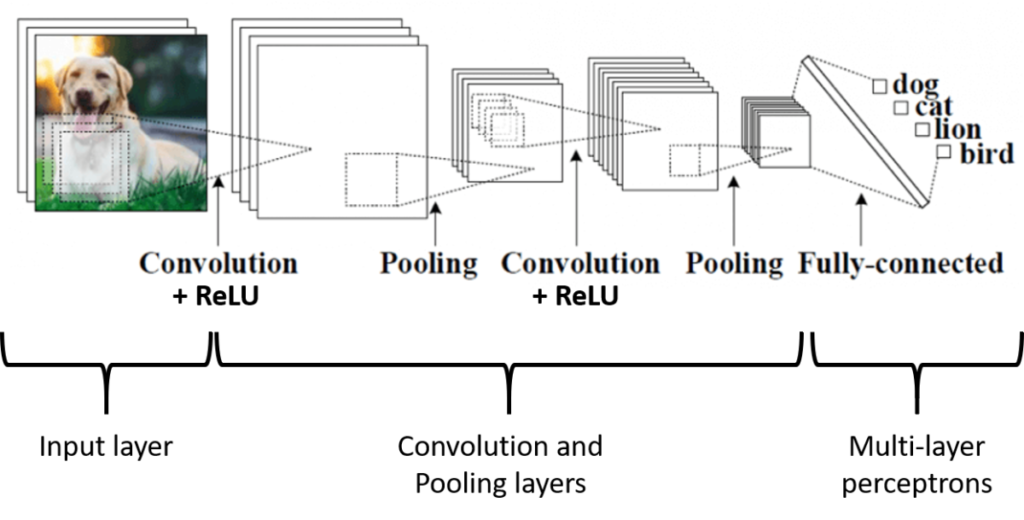
If you are convinced that it takes a particular architecture to work on images, let’s look at what a convolutional neural network architecture looks like (you’ll excuse me, it’s a dog image and not a cat as input…):

Figure 1. Convolutional Neural Networks
Let’s take a relatively classic case study in which we would need to work with neural networks on images: we will try to classify the animal on an input image and we will have to decide if this animal is a dog, a cat, a lion or a bird. The convolutional neural network presented in the figure consists of two large base bricks, one of which you now know! In the first brick, the algorithm will perform successive processing sequences (Convolution – Activation – Pooling) to simplify the input image into characteristics of interest (known as “features”). The extracted characteristics then pass through a multi-layer perceptron architecture in order to produce a classified image. The “only” new thing here is the Convolution – Activation – Pooling part. The network learning mechanisms (forward propagation and backpropagation) remain the same or at least the concepts are the same so I will not go back over them. And it’s the same for solutions to limit overfitting (regularization, dropout…), you already know everything!
I just talked about features, we’ll stop briefly on that. We saw that the limit of multi-layer perceptrons to process images was that the neural model would have too much weight to set up. To limit this number of weights, we will therefore extract important characteristics from the image, which will allow it to be synthesized in a way. And we can then use this synthesis to make our predictions / classifications. The use of features is not new and goes beyond neural networks. In many machine learning methods, when you want to work on images, you extract characteristics manually (for example, texture, boundaries, etc.) beforehand so that you can use these features in classification algorithms. Since these features are expertly selected, it is reasonable to believe that the classification methods should work properly. In the case of convolutional neural networks, the algorithm finds these features of interest on its own! The model finds the features most likely to optimize his classification. Some features may seem relevant to us if we had to look at them with our eye, others may be more surprising. In any case, it must be understood that the use of convolutional neural networks relieves us of this feature extraction step in the sense that this work is performed internally by the algorithm.
Let’s now talk about the passage of the image through the process Convolution – Activation – Pooling :
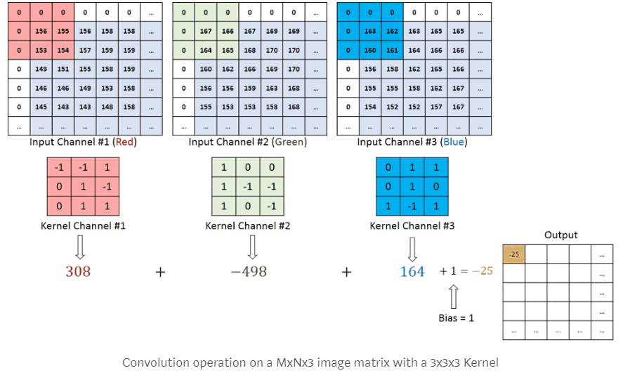
- The Convolution: The convolution step is very classic in image processing (see image below) It consists in moving a filter (or kernel) by dragging it over an image and performing a convolution (a matrix product) of this filter with the underlying image. This filter is nothing more than a square matrix of weights (and these weights will be determined by the gradient descent!). In the image below, we face three pixel tables (the Red, Green and Blue channels), with a filter (kernel) associated with each. Don’t pay attention to the 0 values at the edge, we’ll come back to it later! For the red filter in the upper left corner of the image, the value 308 is obtained by calculating 156-155+153+154 (all other values being 0). For the green filter, the value -498 is obtained by calculating -167-166-165 (all other values being 0). For the blue filter, the value 164 is obtained by calculating 163-160+161.

Figure 2. Convolutional Neural Networks – The Convolution
We see that the 3×3 size filter (9 pixels) transforms the nine pixel values into a single value. Does that mean that applying a convolution will necessarily reduce the size of an image? Yes, unless you add 0s around the original image. You can do the test alone but if you use a 5x5x1 image (a single channel to make it simple) with a 3×3 filter, you will get a 3x3x1 image output. Whereas if you add a 0 pixel outline to the image (as seen in the figure above), you will have an original image of 6x6x1. And if you pass a 3×3 filter, you will have a convolution output image of 5x5x1! This contour of 0 allows to keep the same original image size, which is often interesting! Adding 0s around the image is called Padding. With a padding of 0, no contour of 0 is added. With a padding of 1, one contour of 0 is added. With a padding of 2, two contours of 0 are added, and so on! I told you earlier that during the convolution, the filter was dragged over the entire image but I didn’t tell you how many pixels the filter was shifted as it went along. You can move it one pixel at a time or more! This choice of pixels is called the Stride. With a stride of 1, the filter moves one pixel at a time. With a stride of 2, two pixels at a time. Generally speaking, we choose the stride so that the size of the output image is an integer and not a decimal… With the following formula, you can know the size of the output image of a convolution from the size of the input image (W), the size of the filter (F), the padding (P) and the stride (S):
Size at the end of the convolution = 1 + \frac {W - F + 2P}{S}
For an input image 5×5, a filter 3×3, a padding of 0 and a stride of 1, we obtain an image of size: 1+ (5-3+2*0)/1, or 3 that is an Image 3×3
For an input image 5×5, a filter 3×3, a padding of 1 and a stride of 1, we obtain an image of size: 1+ (5-3+2*1)/1, or 5 that is an Image 5×5
- Activation: In fact, nothing new ! Following a convolution, we often apply an activation function such as ReLU to add a non-linear aspect to our model (you have seen that the convolution was a linear combination of the filter values and the image under the filter). Using the ReLU activation function also allows you to avoid having a negative value on the image at the end of the convolution (I remind you that the ReLU(z)=max(0,z) function)
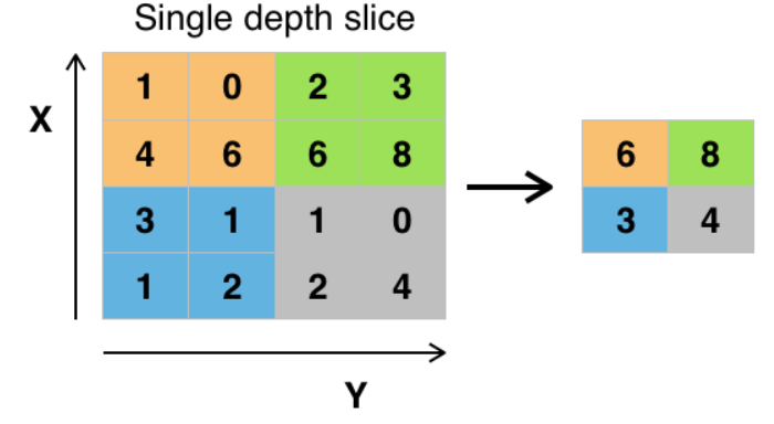
- Pooling: All this is very nice but if we have images at the end of the convolution that are always the same size as the input, we have not solved the problem of the number of weights to set in the model! That’s why a processing sequence ends with a Pooling step. The Pooling step is a sub-sampling step that reduces the size of the image. In the figure below, the Pooling step is performed with a Max filter size 2×2 and a stride size 2 (often the same stride size as the filter size is chosen). That is to say, the image at the output of the convolution is divided into squares of filter size, and in each of the squares, the maximum value under the filter is extracted (we could have used other functions than the Max function!).

Figure 3. Convolutional Neural Networks – Pooling
As we can see on our example of image classification by animal, we can have several Convolution – Activation – Pooling sequences, each with different filter sizes! Often the activation phase is directly linked to the convolution phase. And we can have several Convolution – Activation phases before having a Pooling phase.
When deciding to set up a convolutional neural network to process images, and when you want to have a good prediction/classification quality, you often need many (many) images. And clearly, it can be a problem when you can’t get that many. One of the solutions to help overcome this problem is called Transfer Learning. The idea is to use an existing network that has already learned from a very large image bank (e.g. a Google network) and to refine this network for its own case study. We can indeed imagine that a very large part of the features extracted for this existing network will be useful to us for our own network (and therefore we might as well use it!) What we still have to do is to refine this existing network by changing the last layer of the network, the final classifier (since we will indeed have a different job than the one the network had to do at the beginning – if not use the network directly!) The weights of the previous layers remain unchanged (we use those of the previous network that already extract interesting features) and we only recalculate the weights associated with the last layer of the network to have a network related to our study.
Image Databases
To teach an algorithm to do a task such as recognizing a cat, we said that you need a very large number of images. “No problem! “, you may say. “I have a lot of pictures of my cat, that should be enough to teach a model what a cat is. However, two main problems will arise. First, even if you have made your cat a real photo star, the amount of photos is probably insufficient. Secondly, the diversity of images (different cats,, different backgrounds in the image, several cats in the same image…) is also probably too low. The best algorithm you can create may be good for recognizing your cat from every angle, but it could also fail for the neighbour’s cat. We have already talked about pre-processing algorithms to artificially increase the number of images at our disposal (rotation, distortions…) which is called “data augmentation”. But other solutions exist: image databases.
Image databases are a set of a large number of images grouped into different datasets by specific use cases. Those datasets may be public or not. It is on these immense image databases that very powerful models are trained for, for example, facial recognition to unlock your phone, or even autonomous car guidance. In addition to the fact that the images are of sufficient volume and diversity in the databse, they are also annotated. The annotation consists in filling in each image the characteristic that we want the algorithm to recognize on any image. The annotation is different depending on the use. Let us note for example:
- Image classification so that the algorithm is able to conclude whether or not an image contains a cat. The annotation of the images in the training dataset will consist in having someone to validate that each image that was used an input in the model contains a cat or not.
- The recognition of objects, such as wheat ears in a canopy, to assess one of the components of crop yield. The user annotating this type of image will have to draw the outline of each ear he sees, on each image, so that the algorithm understands what an ear is. It’s already more complicated, isn’t it ?
With these two examples, I think you’re starting to feel that annotating enough images (volume and diversity), one by one, is a titanic task. For this reason, annotated image databases are a considerable asset to those who created them. Just so you know, there are software programs to help with the annotation. For example, some software can detect the contours of shapes, which makes the annotator’s work easier but still requires time and labour (https://hackernoon.com/the-best-image-annotation-platforms-for-computer-vision-an-honest-review-of-each-dac7f565fea)
Although image databases are very precious and sometimes jealously guarded by their creators, there are still quite a few quality public databases that are accessible to everyone. Most often, these “open source” databases are made up of a community of actors (researchers, companies, specialists in birds/flowers/fish…) and it is the contribution of all these actors together that makes it possible to achieve sufficient volumes and quality of images. Let us mention some of these bases:
- “MNIST”: this is a single data set, with images representing handwritten numbers. This very simple dataset (small square grayscale images…) is ideal for starting out in image classification (recognizing each handwritten number) and can be used even with a computer with relatively modest performance
- “ImageNet”: an image bank created by the research community (“WordNet” organization, also known for lexical linguistic databases). The plant world is fairly widely represented, but with an approach that is more related to plants than to crop production
- “Plant Image Analysis”: a databases set up by the world of research to study the different organs (in particular the root and foliar systems) of several commonly cultivated plants
- “Google’s Open Images”: a database set up by Google on which complex models have been trained that can recognize and name several objects in the same image (and not just classify them into a category)
Due to their free nature and their creation by a community, this type of image database can sometimes contain errors (bad annotation, very degraded image quality…). However, these concerns are quite minor in view of the volume of images referenced and because the communities in charge of maintaining these databases regularly update them.
Packages and libraries to use
As the craze for image analysis is very strong at the moment, many methods, packages, libraries have been made available, and one can quickly get lost. Don’t worry! We will present here some packages and reference libraries with which we can already build solid algorithms. I am only considering here the use of Python libraries (you find out for their equivalents in other languages). Here they are:
- Python packages for data manipulation and management (useful for matrices representing images): “Numpy” and “Pandas” are very commonly used in this field
- “cv2” (from its current name in Python): from its real name “OpenCV”, it is a library maintained by Intel providing a large number of features for image and video manipulation (import, display, change of color repository…).
- “Keras”: this library has become a must today, simply because it fulfils its mission well: to make the “engine” that does most of the calculations much easier to use. Without going into detail, the most well-known “engines” are “TensorFlow” (developed by Google), “PyTorch” (used on Facebook) and “CNTK” (developed by Microsoft). Keras comes to fix itself “over” the engine we have chosen (does not work with PyTorch), and allows us to ask for the calculations much more easily than if we made the request directly to the engine.
The tools presented are basic tools; there is no obligation to use them, and there are many other packages and libraries to perform case-specific operations. It must be understood that Keras (or equivalent) is not only an aid to model creation. It is also a great community of people who publish written models that only need to be trained, or even models that are already trained and ready for use (see the transfer learning we have already discussed). This allows us to test many different methods and choose the one that suits us best.
Kaggle Contest
On internet, you will certainly find a large number of sites where attractive names such as “your first neural network in 5 minutes” may attract your attention. But resist the siren songs; these tutorials are generally quite light and include case studies already done and redone. Other more complete tutorials are available, but having already experienced it, it is easy to get discouraged and not go through with such a tutorial (incomplete data, lack of vision on the steps to follow…).
I suggest you take an interest in Kaggle instead. It is a platform on which data analysis competitions are held. The operation is simple: the organizer (a company, a community, a user…) exposes the question to which he would like to find an answer via the competition, he provides a data set (training) to answer it, and he sets the rules (performance criteria to decide between the candidates). Each candidate (individual or team) builds a solution to the question (a model) using the training set and can submit it on the platform for evaluation. Each candidate is free to take up their model if they feel they need to improve it, then submit it one last time before the end of the competition. The evaluation game on which the candidates will actually be ranked is kept secret until the end date of the competition (to avoid overfitting), then the winner is chosen. The competitions revolve around the theme of data analysis, and a significant part of these competitions deals with image processing. Kaggle’s interests are as follows:
- Access to complete annotated data sets
- Reflection on real questions, generally very diversified, which gives a panorama of everything that can be done with the theme of interest (in our case the analysis of images)
- A motivating framework, with a well-designed project: we have the right data, a clear explanation of the problem, in short a course to stay focused from one end to the other
- A very active and motivated community with which to share its progress: forums animated by Internet users show bits of code for such and such an operation, they also share their ideas to improve overall performance… in short, we are never lost on the way to go
First of all, well done if you’ve gotten to that point! Behind the neural networks, we could see that there were a number of concepts, not all of which were always easy to understand. We hear more and more about neural networks because the regression / classification results are quite impressive. The massive use of neural networks is mainly due to the increase in processing capacity allowed by current technological tools and the fact that more and more data are available! Using neural networks requires, as we have seen, adjusting a lot of hyperparameters. There are still quite a few rules of good conduct in the literature or by reusing networks that have worked well! Afterwards, it is up to the user to understand what these hyperparameters are used for in order to adjust them in an intelligent way. One of the problems that still remains with neural networks is their somewhat “black box” effect. It is not always easy to understand how the model learned or what it decided to do to make its prediction. There is active research on this subject……
Some references to look at!
- A set of some videos with very nice illustrations: https://www.youtube.com/channel/UCYO_jab_esuFRV4b17AJtAw
- A very detailed online book on neural networks: http://neuralnetworksanddeeplearning.com/
- Some websites with relevant animations/information:
Support Aspexit’s blog posts on TIPEEE
A small donation to continue to offer quality content and to always share and popularize knowledge =) ?

