Spatial autocorrelation of agronomic and environmental variables

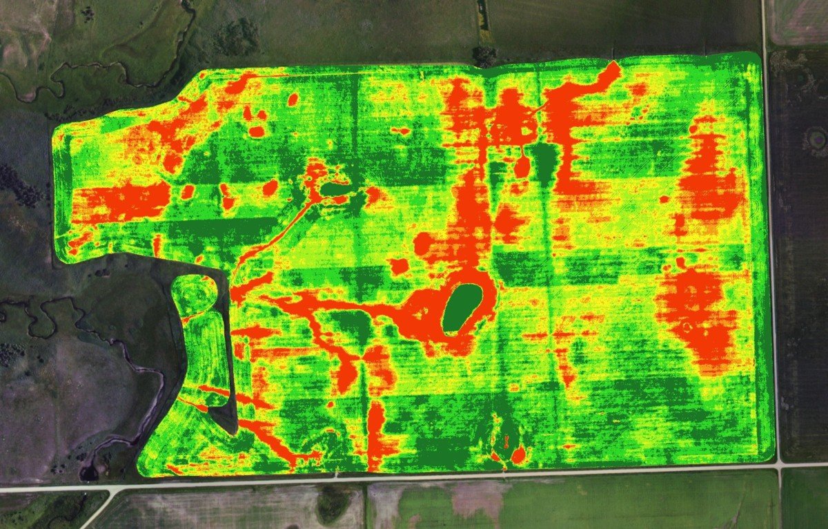
Fig. 1 NDVI spatial pattern within a field

In the fields of agronomy and environment, spatial observations generally exhibit some sort of spatial correlation, to a greater or lesser extent. Spatial data effectively share more similar characteristics with neighbouring observations than with other far apart. This concept has been well described by Tobler (1970) ¹ in its first law of geography : everything is related to everything else, but near things are more related than distant things. Indeed, neighbouring observations are related to more similar topographic, edaphic and climatic factors and as a consequence are more prone to be consistent between each other. This is why spatial patterns or gradient can often be found in agronomic and environmental datasets.

One largely requested analysis in precision agriculture projects is the study of correlations between multiple variables. The objective is generally to find relationships between a parameter A0 that is relatively costly, cumbersome and time-consuming to acquire (ex: water status, leaf nitrogen content…) and other variables that are much cheaper to obtain (ex: NDVI, soil apparent electrical conductivity…). Once these correlations have been clearly defined, it is possible to estimate the variable A0 much more easily.

An inappropriate use of traditional statistical tests in the presence of spatial autocorrelation

Traditional statistical tests such as Pearson’s correlations or ANOVA tests are commonly used to evaluate these correlations. These approaches rely on a strong assumption regarding the independency between the observations of interest. However, as it was previously stated, agronomic spatial datasets are generally autocorrelated which means that this assumption of independency can no longer be tolerated. To be more specific, spatially-correlated observations account for the same piece of information while independent observations characterize a different type of information. As a consequence, the spatial correlation of neighbouring observations will improve the correlations within the datasets while this correlation is only due to the spatial proximity between these observations. If this spatial autocorrelation is not accounted for in these traditional statistical tests, the significativity of the correlations is often overestimated which might lead to misleading conclusions. Taylor and Bates (2013) ² have shown that some correlations between sensor-derived canopy data (NDVI) and vine pruning weights measurements were not significant when considering the spatial autocorrelation of both variables while they were found significant otherwise. This study highlights the importance of considering the autocorrelation of spatial data before performing correlation studies.

How to account for the spatial structure in correlation studies

Dale and Fortin (2002) ³ have proposed an overview of the methods to account for this spatial autocorrelation in correlation studies. Three approaches might be interesting to know about. The first one is relatively simple and consists in the removal of some observations to lessen the autocorrelation within the dataset. Then, the statistical tests can be performed with the newly-defined dataset. The second method aims at reducing the degree of freedom inside the statistical tests. In that case, observations are not removed but the significativity of the correlations is re-evaluated on a much lower number of observations. This approach has the advantage of significantly increasing the p-value of the correlations, hence making the statistical test more robust to spatial autocorrelation. It must be understood that, with this specific approach, the strength of the correlation will not be affected but the p-value associated with the correlation will be much higher than it was before. The last approach mentioned here has to do with randomization or permutation methods. As the name suggests, observations are permuted or switched and correlations tests are performed on the new datasets. This procedure is repeated multiple times to evaluate the significancy of the correlations obtained with the original dataset. In other words, the objective is to check whether the original dataset leads to stronger correlations than the majority of the randomized datasets.

Despite these approaches might have been understood, their implementation might seem much more tricky. In fact, by looking at some listed references (for example those of that gave birth to the second method : Cressie (1990) ⁴; Dutilleul (1993) ⁵), one might be seriously feel helpless. The reference of Dale et Fortin (2002) is more accessible and should help implementing these methods. Concrete examples of the application of these methods can also be found in an article presented at the European Conference on Precision Agriculture (Tisseyre, B., & Leroux, C., 2017). ⁶

Support Aspexit’s blog posts on TIPEEE

---

A small donation to continue to offer quality content and to always share and popularize knowledge =) ?

1. Tobler W., (1970) “A computer movie simulating urban growth in the Detroit region”. Economic Geography, 46(2): 234-240
2. Taylor, J., & Bates, T. (2013). A discussion on the significance associated with Pearson’s correlation in precision agriculture studies. Precision Agriculture, 14, 558-564
3. Dale, M. R. T., and M. J. Fortin. 2002. Spatial autocorrelation and statistical tests in ecology. Ecoscience 9:162–167
4. Cressie, N. A., (1991). Statistics for Spatial Data. John Wiley & Sons, New York
5. Dutilleul, P. (1993). Modifying the t-test for assessing the correlation between two spatial processes. Biometrics, 49, 305–314
6. Tisseyre, B., & Leroux, C. (2017). How significantly different are your within-field zones? Paper presented at the 11th European Conference on Precision Agriculture (ECPA 2017), John McIntyre Centre, Edinburgh, UK, July 16–20 2017, Advances in Animal Biosciences, 8(2), 620-624